← Arsalan Zafar

Proof: MSE makes the Dirac-GAN locally convergent

Generative Adversarial Networks are notoriously unstable due to issues such as mode collapse and training divergence. However, in AI compression, the adversarial training is generally stable and reliable without the necessary tricks such as gradient penalty and adding noise to our input samples. I found this intriguing so I set out to explore why.

One obvious difference is that in compression GANs, we always have access to the ground truth image that we aim to generate. That allows us to use pixel-wise distortion losses in generator (encoder-decoder) training.

Convergence of GANs

Our starting point is the Mescheder et al., 2017 Numerics of GANs paper. We can think of GAN training as a two-player non-cooperative game. The first player is a generator $G_{\theta }(z)$ with parameters $\theta$ that wants to maximize its payoff $g(\theta ,\psi )$, the second player is a discriminator $D_{\psi }(x)$, with parameters $\psi$ that aims to maximize $d(\theta ,\psi )$. The game is at a Nash equilibrium at $({\theta }^{\ast },{\psi }^{\ast })$ when neither player can improve its payoff by changing its parameters slightly. When training approaches a Nash equilibrium and stays there, we can say that it has converged locally.

One method to train a GAN is to use a Simultaneous Gradient Descent, which can be thought of as a fixed point algorithm that applies an operator $F(\theta ,\psi )$ to the parameters of the generator and discriminator $(\theta ,\psi )$ respectively:

$$F(\theta ,\psi )=(\theta ,\psi )+hv(\theta ,\psi ),$$

where $h$ is a learning rate and $v(\theta ,\psi )$ is the gradient vector field, the gradient of each player's payoff with respect to its own parameters:

$$v(\theta ,\psi )=\left[\begin{array}{c}{\mathrm{\nabla }}_{\theta }g(\theta ,\psi )\\ {\mathrm{\nabla }}_{\psi }d(\theta ,\psi )\end{array}\right]$$

Mescheder et al. demonstrate that the convergence near an equilibrium point $({\theta }^{\ast },{\psi }^{\ast })$ can be assessed by looking at the spectrum of the Jacobian of our update operator $F_h^{\prime }(\theta ,\psi )$ at the point $({\theta }^{\ast },{\psi }^{\ast })$:

• If all eigenvalues have absolute value less than 1, the system converges to $({\theta }^{\ast },{\psi }^{\ast })$ with a linear rate (our desired case).
• If there are any eigenvalues with absolute values greater than 1, the system diverges.
• If all eigenvalues have an absolute value equal to 1 (lie on the unit circle), it can be convergent, divergent or neither, but if it is convergent, it will generally converge with a sublinear rate.

For a detailed proof of why the eigenvalues need to lie in the unit circle, see [4], Proposition 4.4.1. This condition translates directly to the eigenvalues of the Jacobian of the gradient vector field $v$. Since $F_h^{\prime }(\theta ,\psi )=I+h{v}^{\prime }(\theta ,\psi )$, the eigenvalues of $F_h^{\prime }$ are $\lambda =1+h\mu$, where $\mu$ are the eigenvalues of $v^{\prime }$. For a small enough positive $h$, exactly when $\mu$ has a negative real part, so we want all eigenvalues of $v^{\prime }$ to have negative real parts.

Now let's look at a toy example to examine the conditions of convergence of GANs and discuss how the AI compression objective impacts convergence. We'll use the Dirac-GAN for simplicity with the non-saturating and vanilla loss for our analysis.

Dirac-GAN

The Dirac-GAN, introduced in [1], consists of a (univariate) generator distribution $p_g={\delta }_{\theta }$ and a linear discriminator $D_{\psi }(x)=\psi x$. The true data distribution $p_D$ is given by a Dirac-distribution concentrated at 0.

Under this formulation, both the discriminator and the generator have exactly one parameter. This simplicity allows us to easily plot the vector field for the GAN in a 2D space to assess convergence behaviour. For a great explanation of vector fields and convergence of GANs, check out this inFERENCe blog post.

The non-saturating GAN generator maximises:

$$g(\theta ,\psi )=f(-\psi \theta )$$

where $f(t)=-\log (1+e^{-t})$. The discriminator maximises:

$$d(\theta ,\psi )=f(\psi \theta )+f(0)$$

where $f(0)=-\log 2$ is a constant. The gradient vector is then:

$$v(\theta ,\psi )=\left[\begin{array}{c}-\psi f^{\prime }(-\psi \theta )\\ \theta f^{\prime }(\psi \theta )\end{array}\right]$$

The system has a unique equilibrium point of the training objective, at point $(\theta ,\psi )=(0,0)$. Indeed, $g(\theta ,0)=f(0)$ and $d(0,\psi )=2f(0)$ are constant for all $\theta ,\psi \in \mathbb{R}$, so neither player can improve its payoff by moving away from 0. Therefore $({\theta }^{\ast },{\psi }^{\ast })=(0,0)$ is a Nash-equilibrium. Now, assuming that $f^{\prime }(0)\ne 0$ we have that $v(\theta ,\psi )=0$ only if $\theta =\psi =0$.

Now we can analyse the convergence of the Dirac-GAN around the equilibrium point $({\theta }^{\ast },{\psi }^{\ast })=(0,0)$ by calculating the Jacobian of the gradient vector field at the equilibrium point:

which has two eigenvalues, $\pm f^{\prime }(0)i$, which are both on the imaginary axis, so the equilibrium is a centre of the vector field [5] and we expect to see a circular vector field. The eigenvalues of $F_h^{\prime }$ are then $1\pm h{f}^{\prime }(0)i$, with absolute value , so simultaneous gradient descent does not converge to the equilibrium. Figure 1 shows that with the non-saturating loss, training spirals towards the equilibrium only very slowly, at a non-linear rate, and does not reach it.

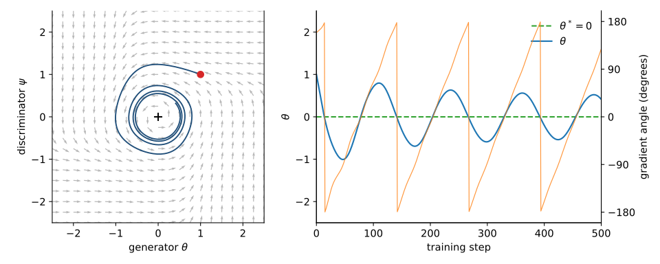
Figure 1: Training behaviour of Dirac-GAN with the non-saturating loss. Left: vector field and the training state of the system visualised for 500 steps (learning rate 0.1); the starting position is marked in red. Right: current value of the generator parameter $\theta$. The green line indicates the value of the ground truth parameter ${\theta }^{\ast }=0$, the blue line shows the estimated $\theta$ and the orange line shows the current angle of the gradient.

Adding MSE

Now, let us look at what happens by adding MSE to the loss for the generator parameters $\theta$. The discriminator's payoff stays the same, but the generator's becomes:

$$g(\theta ,\psi )=f(-\psi \theta )-(0-\theta {)}^2$$

The gradient vector field now has an additional $-2\theta$ term in the $\theta$ partial derivative:

$$v(\theta ,\psi )=\left[\begin{array}{c}-\psi f^{\prime }(-\psi \theta )-2\theta \\ \theta f^{\prime }(\psi \theta )\end{array}\right]$$

The Jacobian of the vector field becomes:

And eigenvalues of the Jacobian of the gradient vector field at the equilibrium point are $-1\pm \sqrt{1-f^{\prime }(0{)}^2}$. Since $f^{\prime }(t)=1/(1+e^t)$, $f^{\prime }(0)=1/2$ and the eigenvalues are $-1\pm \sqrt{3}/2$ (about $-0.13$ and $-1.87$), both of which have negative real parts and 0 imaginary parts, which means that, for a small enough learning rate, the system should be locally convergent around $(0,0)$, an attracting node [5]. The lack of imaginary parts means that there should not be any circular non-convergent behaviour in the gradient vector field, as Figure 2 shows. More generally, with a weight $w$ on the MSE term, the eigenvalues are $-w\pm \sqrt{w^2-f^{\prime }(0{)}^2}$, which have negative real parts for any .

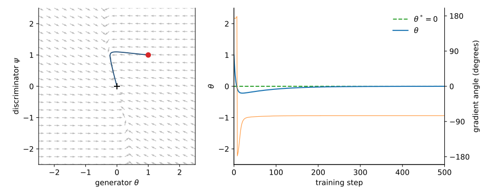
Figure 2: Training behaviour of Dirac-GAN with the non-saturating loss and added MSE, shown as in Figure 1.

Vanilla GAN loss

We can repeat the analysis for the vanilla GAN loss function, where the generator instead minimises the discriminator's payoff, $g(\theta ,\psi )=-d(\theta ,\psi )$. The gradient vector is then:

$$v(\theta ,\psi )=\left[\begin{array}{c}-\psi f^{\prime }(\psi \theta )\\ \theta f^{\prime }(\psi \theta )\end{array}\right]$$

As before, the system has a unique equilibrium point of the training objective at the point $({\theta }^{\ast },{\psi }^{\ast })=(0,0)$, and since $f^{\prime }(-0)=f^{\prime }(0)$, the Jacobian there is the same as for the non-saturating loss, with eigenvalues $\pm f^{\prime }(0)i$. The two losses only differ away from the equilibrium: Figure 3 demonstrates that Dirac-GAN with vanilla GAN loss is divergent around the equilibrium $(0,0)$.

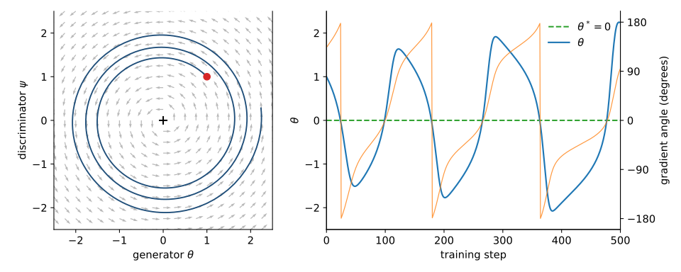
Figure 3: Training behaviour of Dirac-GAN with the vanilla loss, shown as in Figure 1.

However, for similar reasons as above, the behaviour completely changes once we add the MSE component to the generator loss. The gradient vector field now has an additional $-2\theta$ term in the $\theta$ partial derivative:

$$v(\theta ,\psi )=\left[\begin{array}{c}-\psi f^{\prime }(\psi \theta )-2\theta \\ \theta f^{\prime }(\psi \theta )\end{array}\right]$$

and, just like in the case of non-saturating loss, the Jacobian at the equilibrium point is the same as above, with eigenvalues $-1\pm \sqrt{1-f^{\prime }(0{)}^2}$ (Figure 4).

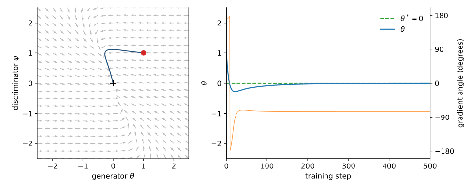
Figure 4: Training behaviour of Dirac-GAN with the vanilla loss and added MSE, shown as in Figure 1.

This analysis shows that adding MSE has the same impact as gradient regularisation and instance noise, which also remove the circular behaviours in the gradient field and force the negative real part in the eigenvalues. In the Dirac-GAN, an $R_1$ gradient penalty [1] with weight $\gamma =2$ gives exactly the same eigenvalues as the MSE, although it acts on the discriminator rather than the generator. This analysis suggests how GANs in compression can sidestep the need for these regularisation methods by simply using the MSE.

Two caveats: this is a local analysis, so it tells us what happens close to the equilibrium, not from an arbitrary initialisation. And in the Dirac-GAN the MSE target is also the only data point, so MSE and the GAN agree on the equilibrium. In compression they generally don't, as the reconstruction with the lowest MSE is blurrier than a realistic one, so adding MSE also moves the point training converges to: the rate-distortion-perception trade-off [6].

Further reading:

• [1] Mescheder, Lars, Andreas Geiger, and Sebastian Nowozin. "Which training methods for GANs do actually converge?." International conference on machine learning. PMLR, 2018. https://arxiv.org/pdf/1801.04406.pdf
• [2] Mescheder, Lars, Sebastian Nowozin, and Andreas Geiger. "The numerics of gans." Advances in Neural Information Processing Systems (2017). https://arxiv.org/pdf/1705.10461.pdf
• [3] Huszár Ferenc "GANs are Broken in More than One Way: The Numerics of GANs." GANs are Broken in More than One Way: The Numerics of GANs. https://www.inference.vc/my-notes-on-the-numerics-of-gans/
• [4] Bertsekas, Dimitri P. "Nonlinear programming." (1999). http://www.athenasc.com/nonlinbook.html
• [5] Theisel, Holger, and Tino Weinkauf. "Vector field metrics based on distance measures of first order critical points." (2002). http://wscg.zcu.cz/wscg2002/Papers_2002/D49.pdf
• [6] Blau, Yochai, and Tomer Michaeli. "Rethinking lossy compression: The rate-distortion-perception tradeoff." International Conference on Machine Learning. PMLR, 2019. https://arxiv.org/abs/1901.07821