Linear attention

Linear attention is becoming the dominant attention mechanism in LLMs. It primarily serves to decouple KV-cache growth from context size (a comparison of softmax attention vs linear attention is provided below). Linear attention belongs in the family of recurrent neural networks and was brought to the forefront by the work Transformers are RNNs in 2020. Its lineage is however deeper, going back to the work on learned associations by Widrow and Hoff, fast weights by Jürgen Schmidhuber and LSTM and RNN work from the late 20th century. Today, we'll look closely at a variant of linear attention, Gated DeltaNet (GDN), the basis of the linear attention layers in the Nenya family of models.

How it works

As opposed to softmax attention, where we matmul $Q$ and $K^{⊤}$ and softmax the resulting matrix and multiply that with the $V$ matrix to get output, in linear attention, we create a state matrix $S$ , into which we write the relationships of $K$ and $V$ (computed by their outer product), and we multiply this $S$ matrix by $Q$ to get our resulting hidden state.

Linear attention revolves around one core entity, the $S$ matrix. We can think of it as a scratch pad. It's a tensor that the model can write into and read from. Each token writes into it and reads from it. $S$ stores information for all previously seen tokens so when decoding a token at position $t$ using $S$ , $t$ will have information about all the tokens up to and including it, but none after it, making it causal.

To add mathematical rigour, the following is the update rule for GDN, given the $k$ , $q$ and $v$ vectors for a token:

\begin{matrix} (1) & S_{t}^{'} = α_{t} S_{t - 1} \end{matrix}

\begin{matrix} (2) & {\hat{v}}_{t} = {S_{t}^{'}}^{⊤} k_{t} \end{matrix}

\begin{matrix} (3) & S_{t} = S_{t}^{'} + β_{t} k_{t} (v_{t} - {\hat{v}}_{t})^{⊤} \end{matrix}

\begin{matrix} (4) & o_{t} = S_{t}^{⊤} q_{t} \end{matrix}

As you can see from the update rules above, we need $k$ , $q$ and $v$ , which are the same vectors we have for softmax attention, produced from multiplying the hidden state of our token with the respective weight matrices. We can also see that we have three new terms, $α$ , $β$ and $S$ and more importantly, a lack of sequence-dependent quadratic operations in the update rule. $α$ and $β$ are the gates which decide how much of $S$ should be kept and how strongly the information stored under $k_{t}$ should be overwritten, respectively.

Eq. 1 decays the existing state $S_{t - 1}$ (empty at the start of a decoding sequence) with $α_{t}$ , which lies between 0 and 1, to gradually forget older $k v$ relationships. Eq. 2 reads what the decayed memory currently stores under the key $k_{t}$ . Eq. 3 writes the correction $v_{t} - {\hat{v}}_{t}$ back under $k_{t}$ as an outer product, scaled by $β_{t}$ (also between 0 and 1) to control the strength of the update. Subtracting ${\hat{v}}_{t}$ is what removes the old information stored under $k_{t}$ . Eq. 4 reads the updated memory with the query to form the output. That is pretty much the crux of linear attention: a matrix we iteratively update with some gates to control reads and writes, and the remaining work goes into ensuring correct initialisations and parameterisations so components are well-behaved at the start of training and throughout it.

Note that the terms read, forget and write here are just matrix multiplications and additions. These are the primitives a model has to read and write from a tensor.

A naive PyTorch implementation

Below is a naive PyTorch implementation (very slow, but helps with understanding) of GDN. The key update rule takes place between lines 126 and 148. However, there are a few important details to understand first:

$α$ has two components: a data-dependent component, computed by passing the input through a linear layer and a softplus, and a data-independent component $A$ which is constant across tokens and learnt over the course of training. The final $α$ combines the two as $α_{t} = \exp (- A \cdot softplus (W_{α} x_{t}))$ , where $x_{t}$ is the token's input and $W_{α}$ the linear layer.
Since $α$ is a forget gate, it must stay between 0 and 1. To achieve this, for the learned parameter component we learn $\log (A)$ (log_alpha in the code), and before applying it to the model, we exponentiate it, which keeps $A$ positive. The softplus keeps the data-dependent component positive too, so their product is positive, and we negate it before exponentiating, which puts $α_{t}$ between 0 and 1.
$S$ is kept per head and is usually a $128 \times 128$ matrix, though this is a hyperparameter.
For $α$ , we have one value per head (which combines the data-dependent and independent components), per token, and before applying it to the $S$ matrix, we broadcast it to a $128 \times 128$ matrix, making it a coarse gate.
$β$ is also one value per head, but it only has a data-dependent component and we use a linear layer to compute it. To squeeze the values between 0 and 1, we use a sigmoid on the outputs of the linear layer.
Both $α$ and $β$ vary per token, but $S$ is persistent between tokens.
We store $S$ as keys × values, built from outer products $k v^{⊤}$ ; you will also see it stored as values × keys ( $v k^{⊤}$ ) sometimes, which transposes every product in the update rule but leaves the logic unchanged.
There are 1D depthwise convolutions used in popular implementations to help with local token mixing before the linear attention operations, and these act on the $K$ , $Q$ and $V$ matrices. These are depthwise, so weights across the feature dims of a single token (d_out in the code) of $K$ , $Q$ and $V$ are independent. We transpose $K$ , $Q$ and $V$ to make d_out the 'channel' dim so depthwise conv treats them with separate kernels. For example, the conv would take the first feature dim of $K$ , which would be a $[t, 1]$ vector, and convolve this with a 1D kernel. This would take 4 neighbouring tokens at a time and produce a single value, and then with stride 1, slide forward by one token. Finally, to preserve dimensions and causality, we left-pad, which means the oldest token gets three zeros as context in its kernel of size 4 and all convolutions remain causal.
After the convolutions, we scale each query and key to unit length (F.normalize in the code), so that $k^{⊤} k = 1$ . This is what makes Eq. 3 a step of size $β_{t}$ towards $v_{t}$ : with a longer key, reading it back after a write would return ${\hat{v}}_{t} + β_{t} ‖ k_{t} ‖^{2} (v_{t} - {\hat{v}}_{t})$ , which overshoots $v_{t}$ once $β_{t} ‖ k_{t} ‖^{2} > 1$ and can make the state blow up over many tokens. Scaling the query as well keeps the read-out of Eq. 4 on a fixed scale, while the values only get an RMSNorm, which fixes their scale without making them unit length.
There is an output gate which is input-dependent to add expressivity.


class GatedMultiHeadDeltaAttention(nn.Module):
    def __init__(self, d_model, d_out, context_length, dropout, num_heads, qkv_bias=False):
        super().__init__()

        self.d_out = d_out
        self.num_heads = num_heads
        self.head_dim = d_out // num_heads

        # Q, K, V projections
        # [b, t, d_model] @ [d_model, d_out] -> [b, t, d_out]
        self.W_query = nn.Linear(d_model, d_out, bias=qkv_bias)
        self.W_key = nn.Linear(d_model, d_out, bias=qkv_bias)
        self.W_value = nn.Linear(d_model, d_out, bias=qkv_bias)

        # Output projection to mix information between heads
        # [b, t, d_out] @ [d_out, d_out] -> [b, t, d_out]
        self.out_proj = nn.Linear(d_out, d_out)

        # Update gate, one scalar per token per head
        # [b, t, d_model] @ [d_model, nh] -> [b, t, nh]
        self.beta = nn.Linear(d_model, num_heads)

        # Input-dependent forget gate, one scalar per token per head
        # [b, t, d_model] @ [d_model, nh] -> [b, t, nh]
        self.alpha = nn.Linear(d_model, num_heads)

        # Input-dependent output gate, applied after combining heads
        # [b, t, d_model] @ [d_model, d_out] -> [b, t, d_out]
        self.gate = nn.Linear(d_model, d_out)

        # Input-independent forget gate, one parameter per head
        # [nh]
        self.log_alpha = nn.Parameter(
            torch.log(torch.empty(num_heads).uniform_(0, 16))
        )

        # Depthwise causal convolutions for local token mixing
        # Input: [b, d_out, t + 3] -> Output: [b, d_out, t]
        self.conv_k = nn.Conv1d(
            d_out, d_out, kernel_size=4, stride=1, groups=d_out
        )
        self.conv_v = nn.Conv1d(
            d_out, d_out, kernel_size=4, stride=1, groups=d_out
        )
        self.conv_q = nn.Conv1d(
            d_out, d_out, kernel_size=4, stride=1, groups=d_out
        )

        # RMS normalization over head dimension
        self.norm = nn.RMSNorm(self.head_dim, eps=1e-6)

    def forward(self, x):
        b, num_tokens, d_model = x.shape  # [b, t, d_model]

        # Project input into Q, K, V
        # [b, t, d_model] @ [d_model, d_out] -> [b, t, d_out]
        keys = self.W_key(x)
        queries = self.W_query(x)
        values = self.W_value(x)

        # Left-pad by 3 tokens for causal convolution
        # [b, t, d_out] -> [b, t + 3, d_out]
        keys = F.pad(keys, (0, 0, 3, 0, 0, 0))
        queries = F.pad(queries, (0, 0, 3, 0, 0, 0))
        values = F.pad(values, (0, 0, 3, 0, 0, 0))

        # Apply depthwise convolutions followed by SiLU
        # [b, t + 3, d_out] -> [b, d_out, t + 3]  (transpose)
        # [b, d_out, t + 3] -> [b, d_out, t]  (conv, then SiLU)
        # [b, d_out, t] -> [b, t, d_out]  (transpose back)
        keys = F.silu(self.conv_k(keys.transpose(1, 2))).transpose(1, 2)
        queries = F.silu(self.conv_q(queries.transpose(1, 2))).transpose(1, 2)
        values = F.silu(self.conv_v(values.transpose(1, 2))).transpose(1, 2)

        # Split embedding dimension into heads
        # [b, t, d_out] -> [b, t, nh, hd]
        keys = keys.view(b, num_tokens, self.num_heads, self.head_dim)
        queries = queries.view(b, num_tokens, self.num_heads, self.head_dim)
        values = values.view(b, num_tokens, self.num_heads, self.head_dim)

        # Move head dimension before sequence dimension
        # [b, t, nh, hd] -> [b, nh, t, hd]
        keys = keys.transpose(1, 2)
        queries = queries.transpose(1, 2)
        values = values.transpose(1, 2)

        # Unit-length Q and K (so k^T k = 1); RMSNorm on V
        # [b, nh, t, hd] -> [b, nh, t, hd]
        keys = F.normalize(keys, dim=-1)
        queries = F.normalize(queries, dim=-1)
        values = self.norm(values)

        # Initialize recurrent state matrix S_0
        # [b, nh, hd, hd]
        S = x.new_zeros(b, self.num_heads, self.head_dim, self.head_dim)

        # Compute input-dependent component of forget gate
        # [b, t, d_model] @ [d_model, nh] -> [b, t, nh]
        input_dependent = F.softplus(self.alpha(x))

        # Compute input-independent component of forget gate, A = exp(log_alpha)
        # [nh] -> [1, 1, nh]
        A = self.log_alpha.exp().unsqueeze(0).unsqueeze(0)

        # Combine forget gate components
        # [b, t, nh] * [1, 1, nh] -> [b, t, nh]
        log_combined = -input_dependent * A

        # Exponentiate to obtain alpha in (0, 1]
        # [b, t, nh] -> [b, t, nh]
        alpha_final = log_combined.exp()

        # Compute update gate beta
        # [b, t, d_model] @ [d_model, nh] -> [b, t, nh]
        beta = torch.sigmoid(self.beta(x))

        # Compute output gate
        # [b, t, d_model] @ [d_model, d_out] -> [b, t, d_out]
        gate = self.gate(x)

        # Collect token outputs from recurrent state updates
        outputs = []

        # Process tokens sequentially: each step below is one of Eqs. 1-4
        for i in range(num_tokens):

            # Current token's vectors and gates
            # [b, nh, t, hd] -> [b, nh, hd];  [b, t, nh] -> [b, nh, 1, 1]
            q, k, v = queries[:, :, i], keys[:, :, i], values[:, :, i]
            alpha_i = alpha_final[:, i, :, None, None]
            beta_i = beta[:, i, :, None, None]

            # Eq. 1, decay: S' = alpha * S
            # [b, nh, 1, 1] * [b, nh, hd, hd] -> [b, nh, hd, hd]
            S = alpha_i * S

            # Eq. 2, read what S' stores under k: v_hat = S'^T k (computed as the row k^T S')
            # [b, nh, 1, hd] @ [b, nh, hd, hd] -> [b, nh, 1, hd] -> [b, nh, hd]
            v_hat = (k.unsqueeze(-2) @ S).squeeze(-2)

            # Eq. 3, write the correction under k: S = S' + beta * k (v - v_hat)^T
            # [b, nh, hd, 1] @ [b, nh, 1, hd] -> [b, nh, hd, hd]
            S = S + beta_i * (k.unsqueeze(-1) @ (v - v_hat).unsqueeze(-2))

            # Eq. 4, read the updated memory with the query: o = S^T q (as the row q^T S)
            # [b, nh, 1, hd] @ [b, nh, hd, hd] -> [b, nh, 1, hd]
            outputs.append(q.unsqueeze(-2) @ S)

        # Concatenate outputs along sequence dimension
        # t x [b, nh, 1, hd] -> [b, nh, t, hd]
        # [b, nh, t, hd] -> [b, t, nh, hd]
        context_vec = torch.cat(outputs, dim=2).transpose(1, 2)

        # Normalize output over head dimension
        # [b, t, nh, hd] -> [b, t, nh, hd]
        context_vec = self.norm(context_vec)

        # Combine heads into embedding dimension
        # [b, t, nh, hd] -> [b, t, d_out]
        context_vec = context_vec.reshape(b, num_tokens, self.d_out)

        # Apply input-dependent output gate
        # [b, t, d_out] * [b, t, d_out] -> [b, t, d_out]
        context_vec = context_vec * F.silu(gate)

        # Final projection to mix information between heads
        # [b, t, d_out] @ [d_out, d_out] -> [b, t, d_out]
        context_vec = self.out_proj(context_vec)

        return context_vec

In a serious training run, it's recommended to use the optimised version in the fla library which has an extraordinary amount of work poured into it, along with a few tricks to optimise the token-wise read–write loop seen in the code above.

Results

Below is a comparison of validation loss (held-out cross-entropy) between a softmax transformer and GDN (with parameter parity) trained for 2.5B tokens on FineWeb-Edu and evaluated on a held-out subset of it. As you can see, there is a ~5% improvement (which is quite large w.r.t. other architecture improvements). However, we have to be careful, as this is a 124M model, with 2.5B tokens and gaps can close with more training.

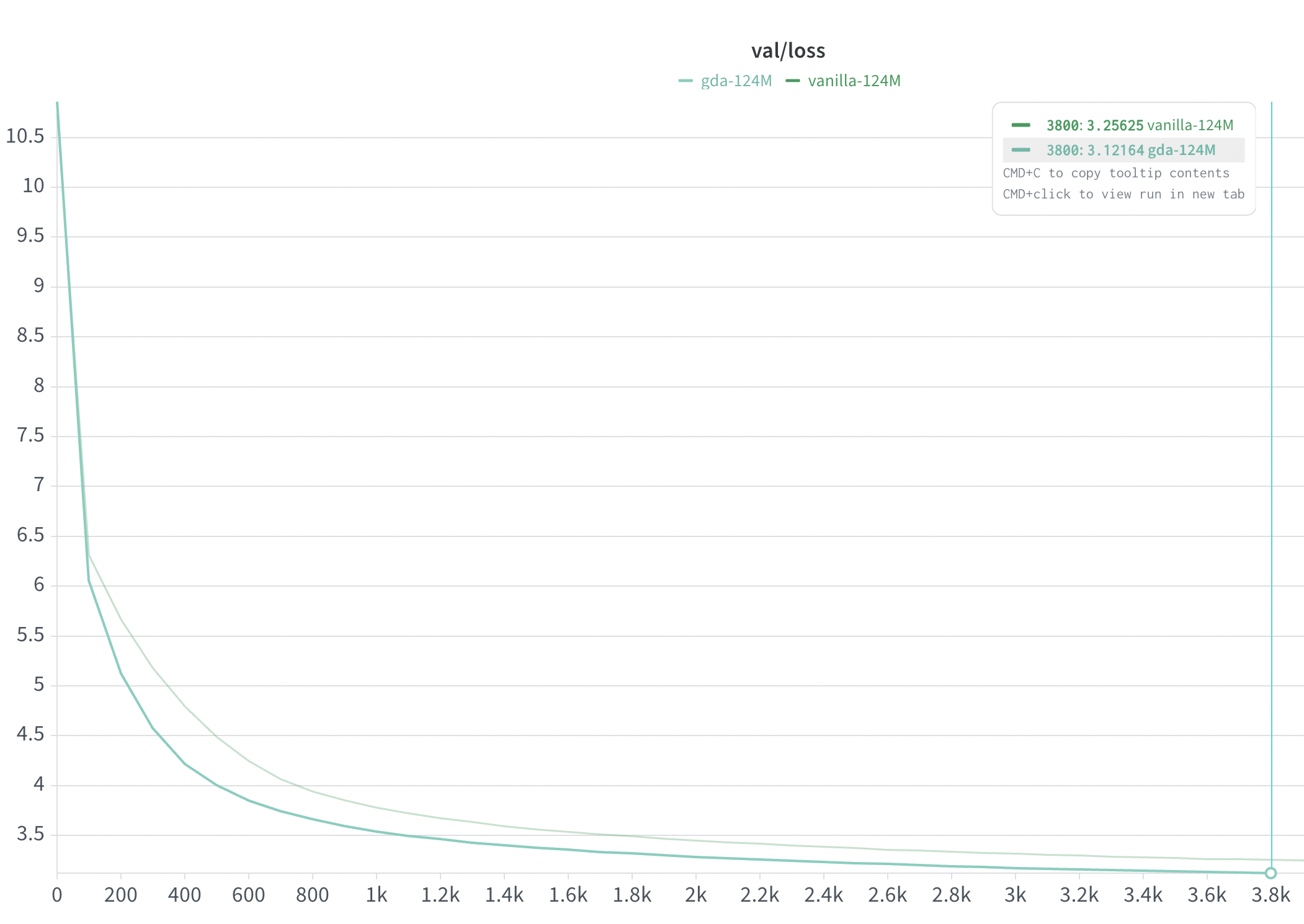
Figure 1: Held-out validation loss comparing softmax and GDN attention mechanisms.

Cache size and FLOP growth

Assume we have $L$ layers in our network, the context length is $t$ and $d_{m o d e l}$ is our model dimension (the feature size of the $K$ , $Q$ and $V$ matrices). The size of KV cache growth for softmax attention is then $2 L t d_{m o d e l}$ since every new token needs all the previous $k$ vectors to compute attention again, and the output needs all the previous $v$ vectors to apply the attention to and form the output. The factor of 2 comes from having to store both $K$ and $V$ .

In contrast, for GDN, the cache scales with $L n_{h e a d s} d_{h e a d}^{2}$ where $d_{h e a d}$ is the head dimension, usually 128, and $n_{h e a d s}$ is the number of heads, a hyperparameter set during model design. $d_{h e a d}$ is a constant and so is $n_{h e a d s}$ , and the entire term is independent of $t$ , the context length. Each new token only needs the previous state matrix $S$ , which is defined per head, which uses a fraction of the memory.

The FLOPs required for the attention operation also scale favourably for linear attention. For softmax, the FLOPs for attention scale quadratically with the context size, $L t^{2} d_{m o d e l}$ , since we must compare each token to every other token and the comparison is between $d_{m o d e l}$ values. GDN on the other hand, scales linearly with the number of tokens, $L t n_{h e a d s} d_{h e a d}^{2}$ , as there is no token-to-token comparison but rather a single matrix that every token writes into and reads from, which has dimensions $d_{h e a d} \times d_{h e a d}$ , and there are $n_{h e a d s}$ of them.

Method	Memory scaling	Attention FLOPs	Loss delta
Softmax	$2 L t d_{m o d e l}$	$O (L t^{2} d_{m o d e l})$	0.0%
GDN	$L n_{h e a d s} d_{h e a d}^{2}$	$O (L t n_{h e a d s} d_{h e a d}^{2})$	−5%

These amazing features of linear attention aren't free. Since we don't keep exact $k$ and $v$ vectors of previous tokens, recall over longer contexts is a known issue of linear attention. The solution to this problem is to mix softmax attention layers with linear attention, which significantly reduces cache size while maintaining long-context performance. Just as in other popular architectures like Kimi K3, Nenya has its first and last layers as Multi-head Latent Attention (MLA), giving a ~5.5× compression, and every 4th layer is MLA too, with all other layers being linear attention built on GDN.