← Arsalan Zafar

Nenya technical report

Nenya is a general purpose 0.5B active, 2.5B total parameter mixture-of-experts (MoE) base model. Nenya rivals Qwen3.5 2B on pretraining benchmarks with 500× lower training compute and 3.4× fewer active FLOPs/token. In this report, we share architecture details, model behaviour throughout training, benchmarks, insights into our runtime optimisations, and our training and data configurations. The model and the Mac implementation are available to play with through Hugging Face, as well as with pip install "nenya[mac]".

Model: https://huggingface.co/ArsalanZ/Nenya-2.5B-A0.5B-Base

Mac engine: https://huggingface.co/ArsalanZ/Nenya-2.5B-A0.5B-Base-Metal-8bit

Architecture overview

The architecture is the classical stack of token mixer and feed-forward transformer blocks that seamlessly incorporates mHC, Engram and MoE. Figure 1 shows the complete architecture.

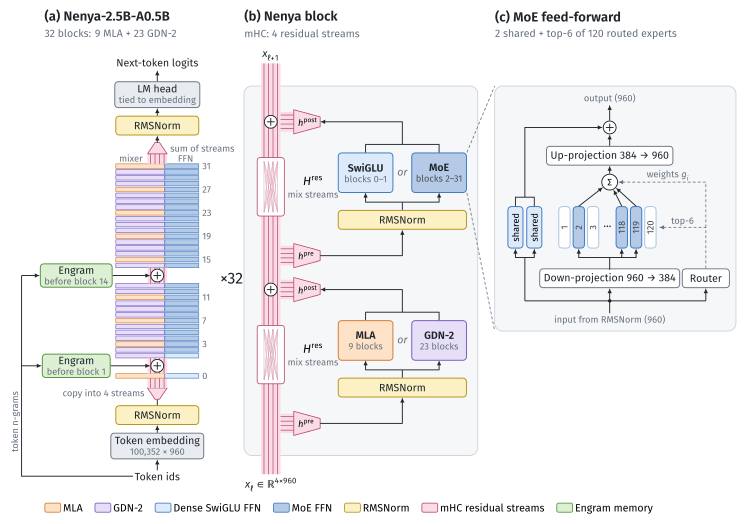
Figure 1: Nenya-2.5B-A0.5B detailed architecture diagram. All feed-forward blocks, including the experts, the shared experts and the dense feed-forward of blocks 0 and 1, are SwiGLU-style feed-forward networks.

Input text is tokenised with the Olmo 3 tokeniser and the embeddings are copied into four mHC residual streams and fed into the first transformer block. Each transformer block consists of a token mixer and a feed-forward MoE layer. Before each sublayer, there is a read operation, $H^{pre}$, from the residual stream and a write operation, $H^{post}$, after it, which allows each sublayer to read and store specific information in the residual streams. For the token mixer sublayer, most layers are linear attention to curb KV cache growth while the first, the last and every 4th are Multi-head Latent Attention (MLA) modules, to preserve long-context recall. The MoE sublayer consists of 120 latent experts for each layer, and each token uses 2 full-dimension shared experts and 6 latent routed experts. The first two layers are dense feed-forward layers. Finally, a bigram and trigram vector is added to each token's value of the residual stream after the first layer and the 14th layer.

Attention

Nenya uses two classes of token mixers, MLA and Gated DeltaNet-2. Figure 2 shows how we set up the Gated DeltaNet-2, while Figure 3 shows our MLA configuration.

Linear attention revolves around one core entity, the $S$ matrix. We can think of it as a scratch pad. It's a tensor that the model can write into and read from. Each token writes into it and reads from it. $S$ stores information for all previously seen tokens so when decoding a token at position $t$ using $S$, $t$ will have information about all the tokens before it, making it strictly causal. Figure 2 demonstrates the inner workings of GDN-2 and Appendix A13 gives the details, while the linear attention blog explains GDN-1 in detail.

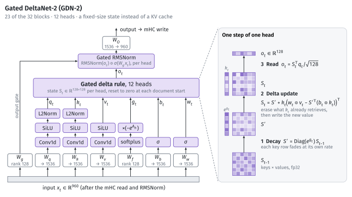
Figure 2: GDN-2 keeps a 128 × 128 state per head. Each token decays it per key channel, erases what the key already retrieves and writes the new value.

For MLA, the read from mHC is projected up by $W^Q$ to a query tensor and projected down by $W^{DKV}$ to a KV storage tensor. The KV tensor is stored in the cache and it's 3× smaller than the hidden states, and since it's shared between the key and value tensors, it leads to a total of ~5.5× savings in KV storage, counting the 32 values described next. We also break off 32 values directly from the output of $W^{DKV}$ and skip them to the keys. This is to guard against loss of context if we apply any extreme KV cache quantisation as it allows the network to skip full-precision information to $k$ and $q$. The KV storage tensor is then projected up to get our key and value tensors to compute standard softmax attention. There is also an additional gated projection $W^G$ applied element-wise at the output of MLA to avoid attention sinks.

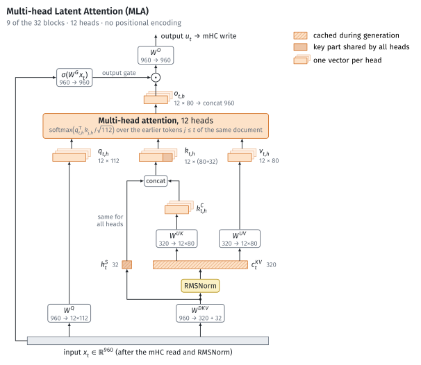
Figure 3: MLA caches a 320-d latent and a 32-d key shared by all heads: 352 numbers per token per layer. $\sigma$ here is the sigmoid function.

mHC

Manifold-constrained hyper-connections (mHC) turn the vanilla single-channel residual stream into $n$ streams and allow sublayers to write into and read from the streams the information they please. This gives the model more control over the residual stream while increasing its capacity. mHC was introduced by DeepSeek and the inner workings of mHC are detailed in our blog: Manifold-constrained hyper-connections.

Figure 4a looks at how stream spread varies with training. It's measured on the last block before the streams are summed and it's a measure of how different the streams are from each other, intended to measure stream collapse. We observe that the stream spread levels off to 0.3 after 20B tokens. This suggests that the extra channels are being useful and the model is putting different information in them.

Figure 4b compares the output of the sublayer with what's written into the stream by simply taking the ratio of RMS of the sublayer output and the stream write. We can see that attention output gets written into the stream at the same scale as its output, but feed-forward layers need to be scaled down as they are 2–6× larger so $H^{post}$ acts as a learned gain. For Gated DeltaNet-2, the penultimate layers give the output of each head an RMS of 1 and a sigmoid gate is applied to it which helps bound the scale, while MLA is bounded by softmax as well as a sigmoid gate. However, the MoE module chains many unbounded matrices together, as well as a weighted sum of 6 experts and the scale is the product of these leading to large values being output. This shows that the MoE layers need an RMSNorm after the layer output, as is often used in other architectures, which would give the feed-forward layers a higher effective learning rate as the scale of the updates would be closer to the scale of parameters being updated.

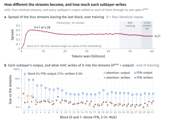
Figure 4: How different the four mHC residual streams become, and how much each sublayer writes into them. (a) The stream spread (metric in Appendix A1). (b) Each sublayer's output (hollow) and what mHC's write gate $H^{post}$ adds of it to the streams (filled), both relative to the streams' size. Attention output is written at about its own size (median ×0.97; only blocks 1–3 are scaled down, to ×0.22–0.37). The FFN outputs are far larger, 315× the streams in block 0, about 77× in blocks 1–2 and 2–6× from block 10 on, and $H^{post}$ scales them down 6–1,000×, so each FFN adds 0.1–1.2× the streams' size.

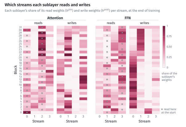
Figure 5: Which of the four streams each sublayer reads and writes: each sublayer's share per stream of its read weights ($H^{pre}$) and write weights ($H^{post}$), at the end of training (metric in Appendix A2). The rings mark the one stream each sublayer read at initialisation, cycling with depth (the writes start equal on all four streams); training moved about half of the reads.

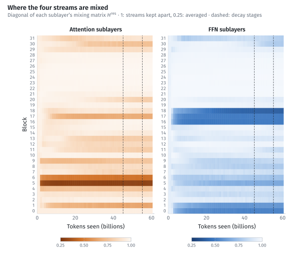
Figure 6: Where the four streams are mixed: mean of $H^{res}$'s four diagonal entries over tokens (metric in Appendix A3), attention sublayers on the left, FFN sublayers on the right. Every matrix starts close to the identity (diagonal 0.95).

Figure 5 shows which stream each sublayer reads from and writes into to assess stream specialisation. We can see a few patterns emerging:

• Both feed-forward and attention sublayers treat stream 2 as read-only.
• The feed-forward outputs written into stream 2 by blocks 0 and 1 are carried to the end, where they are heavily read by the attention sublayers from block 20 onwards, acting as a skip connection. This is likely the embedding vector being skipped deeper into the network: in other words, the 'embedding lane'.
• FFN sublayers treat streams 0 and 1 as write lanes, writing into stream 0 in the early and middle blocks and stream 1 in the late blocks. They treat streams 2 and 3 as the main read lanes.

Figure 6 shows the intensity of mixing across the blocks, per sublayer. It's the diagonal value in the mixing matrix, and 0.25 means complete averaging while 1 means zero mixing. The strongest mixing appears early in training: block 5's attention reaches 0.35 by 2.1B tokens, close to averaging all four streams, and the FFNs of blocks 16–17 and of the dense blocks 0–1 fall to 0.5–0.7 by 10B. For a few sublayers, mixing gets stronger with training: block 18's FFN (0.59 at 10B, 0.39 at the end), and, in the last blocks, block 30's attention (from 0.93 to 0.73) and its FFN (from 0.96 to 0.78), mostly late in pretraining and in midtraining. Interestingly, blocks 21–28 keep their streams apart throughout (≥ 0.95). Finally, there doesn't seem to be any visible pattern between mixing and reading from or writing to the residual streams.

From this, we can argue that the model is using the residual streams well by specialising them for reads and writes and keeping one as the embedding lane, while the mixing is more clustered than anticipated and has no obvious pattern. A downside of mHC is that it makes inference tedious as it introduces operations before and after sublayers. In our optimisations, we found mHC kernel launch overhead to be one of the main bottlenecks.

Engram

We follow the Engram approach of DeepSeek. We create bigram and trigram hashes from the token sequence, which hash into 8 bigram and 8 trigram tables respectively and fetch a total of 16 embedding vectors. These embedding vectors are projected to key and value vectors, and the key is dotted with each residual stream to give $\alpha$, a scalar sigmoid gate for the embedding vector, which is used to gate $v$ before adding it into the hidden states. Since we have four streams, we have four separate key projections, resulting in four $\alpha$ values so the model can control what Engram information should go into what stream. A more detailed explanation of the inner workings of Engram is available in our blog here: Engram.

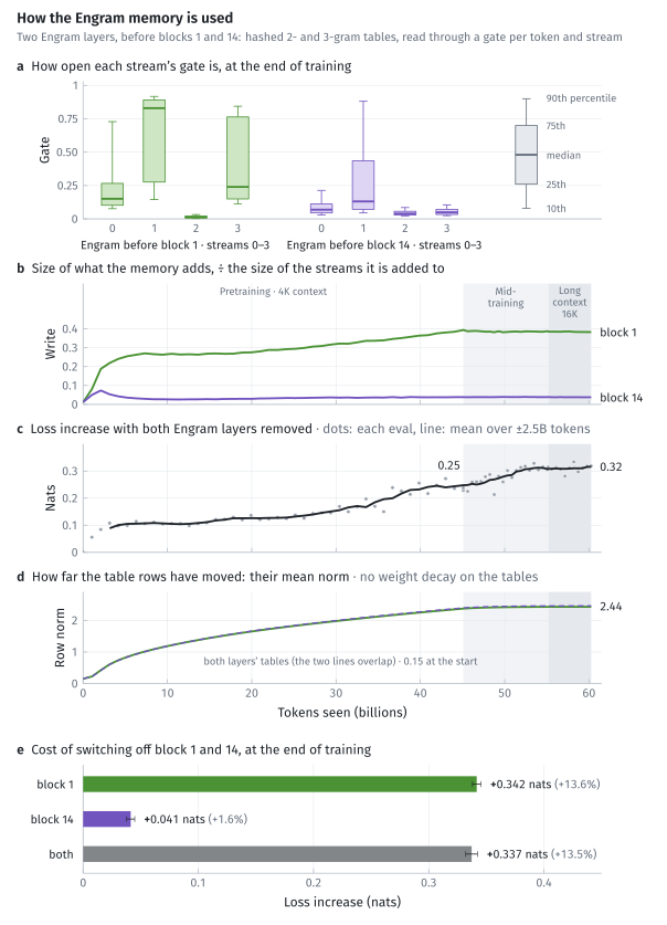
Figure 7: How the Engram memory is used. (a) How open the gates are (the $\alpha$ value) for each stream and block at the end of training. (b) At the end of training, memory before block 1 adds 38% of the streams' size, the one before block 14 adds 4% (metric in Appendix A4). (c) The model leans on the memory more as training goes on: removing both Engram layers costs 0.10 nats at 4B tokens, 0.25 at the end of pretraining and 0.32 at the end. (d) With no weight decay and 5× the AdamW learning rate, the table rows keep moving through pretraining, their mean norm (metric in Appendix A5) growing from 0.15 to 2.38, and barely move in the LR decay. (e) The cost of switching off each block separately, at the end of training.

Figure 7a shows how open the gate $\alpha$ is for both Engram layers, for each of the residual streams of mHC, where 1 represents fully open and 0 is fully closed, telling us how much of the Engram information the model wants to keep. On average across the gates, block 1's $\alpha$ is at 0.33 while block 14's is at 0.14, suggesting the model wants to lean more heavily on the memory in the earlier layer than the later one. We also see this showing up in Figure 7b, where block 1's Engram accounts for ~38% of the magnitude written into the stream, while block 14's accounts for 4%. Looking at the impact on loss of switching off a block's Engram in Figure 7e, we also see block 1 being 8× more costly. This suggests that block 14's Engram is not as effective and we could save ~264M parameters at the cost of a 1.6% higher validation loss.

From Figure 7a, it is also clear that both blocks respect mHC stream 2 as the clean embedding skip lane and treat it as read-only, as the gates are almost closed here. Block 1 treats streams 0, 1 and 3 as the main write lanes it writes into, while block 14 writes mainly into streams 0 and 1.

From Figures 7c and 7d, we can see that the tables are learning throughout training. The L2 norm of the rows increases with training, growing a total of 16×, and the total cost of switching off both Engram blocks also rises with training and continues to do so. By the end, it costs about 13% of the total loss and is still increasing.

In summary, Engram seems to be very important for modelling capacity but would benefit from further ablations on where it should be placed deeper in the network. During inference, it is also very cheap as it's a lookup that can be pipelined with the attention and FFN layers.

MoE

Our MoE architecture is the fine-grained latent MoE architecture introduced in Kimi K3. We use 120 SwiGLU latent routed experts and two full-dimension SwiGLU shared experts. The final output is the sum of these. To stabilise the MoE during training, we use quantile balancing, as introduced by Kimi K3 and explained in our blog Quantile balancing. Figure 1c outlines the architecture in more detail.

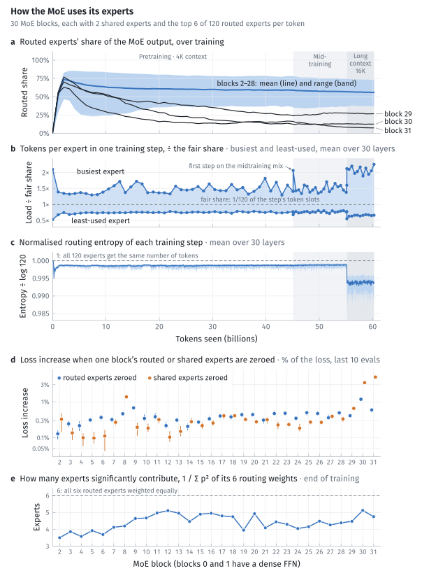
Figure 8: How the MoE uses its experts. (a) The routed experts' share (metric in Appendix A6) settles at 37–73% in blocks 2–28, while blocks 29–31 move to their shared experts: block 31's routed share falls from 63% to 7%. (b) The busiest expert (metric in Appendix A7) gets 1.43× its fair share and the least-used 0.75×. (c) The routing entropy (metric in Appendix A8) stays close to its maximum of 1: a median of 0.999 in pretraining and 0.994 in long context, as even as 119 and 116 equally used experts. (d) What zeroing a block's shared or routed experts costs, as a percentage of the loss. (e) The top routing weight (metric in Appendix A9) takes 29–49% of a token's six, so 3.5–5.1 experts act per token, fewest in the first MoE blocks.

Figure 8a shows the routed experts' share of the MoE output, which tells us how dominant they are as training progresses. For blocks 2–28, by the end of the 60B tokens, the routed share is about 50% of the final output, while for blocks 29–31 the routed share is below 25% of the MoE output, and block 31's routed share is 7% of the output. This measure of course doesn't point to usefulness, as we see from Figure 8d, but rather to how dominant the routed experts are.

Figure 8b shows how tokens in one training step are distributed across the experts. Given that we have 120 experts, each expert's fair share is 1/120 of the step's token slots. We find that the busiest expert gets 1.43× its fair share while the least busy expert gets 0.75× its fair share, and no expert goes without token allocation in any training step. We also notice that in long-context training, the spread between the busiest and least busy experts increases since more of the data is from a single source. Figure 8c shows the routing entropy, which stays close to the ideal value of 1. This points against any expert collapse during training.

Figure 8d shows how much the loss increases if we zero out either the shared-expert or routed-expert component of our MoE to help us assess their relative importance. We can observe a few patterns:

• It's clear that both the shared and the routed experts contribute to loss improvement.
• The contribution of both MoE components increases as we get deeper in the network.
• Routed experts (blue dots) for the majority of the blocks contribute more than the shared experts (orange dots).
• For blocks 30 and 31, the shared expert component contributes 3.5% and 4.9% of the loss, noticeably more than the routed component, likely due to their proximity to the output.

Since each of the experts is weighted by the softmax of router logits, Figure 8e shows how many experts contribute significantly, which tells us whether the router actually wants to use the experts it selects since quantile balancing could be forcing even selection, while the router could be switching them off with softmax weights. We can see that in the earlier layers, the top expert carries most of the weight, but with depth, we see roughly 4 active experts holding most of the weight, which is acceptable given each token picks 6.

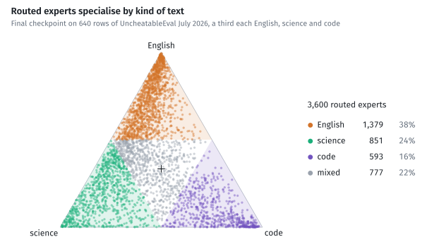
Figure 9: How the routed experts specialise by kind of text (metric in Appendix A10).

From Figure 9, we can see that our experts also specialise well across different domains such as English, science and code. Most specialise in English and science as that is the majority of our training data.

In summary, the model is utilising the shared and routed experts well with no apparent collapse. Switching off all shared experts across the network costs 104% of the val loss while switching off all routed experts costs 69% of the loss. The experts are also specialising in different domains, a behaviour we hoped to achieve.

Training schedule

Our training schedule consists of three stages: pretraining, midtraining and long-context training. These stages vary by the number of tokens they receive, context size and the LR regime. Pretraining lasts 45B tokens at peak LR, after 2B warmup tokens. At 45B, we kick in high-quality midtraining data and start to decay the LR with a $1-\sqrt{t}$ schedule for 15B tokens, and the last 5B tokens go to long-context training, where we continue the $1-\sqrt{t}$ decay from the midtraining stage, but change data sources to long-context data and increase the context size to 16K.

For our optimisers, we use AdamW and Muon as well as MuonBatched for the routed experts to make training efficient. Our experts are stored as 3-D tensors (of shape [120, 384, 768] for w_gate_up) so we can use batched matmul for faster computation. torch.optim.Muon is unable to handle these tensors and flattening to 2-D matrices would apply orthogonalisation incorrectly, so MuonBatched exists to handle this scenario. The first table lists the optimiser groups, their parameters and learning rates; the second, the training stages.

Optimiser	Group	What is in it	Parameters	Peak LR	Weight decay
Muon	2-D matrices	GDN-2 projections, experts, MLA, dense FFNs of blocks 0–1, Engram key/value projections, mHC mixing matrices	373.3M (14.4%)	3×10⁻³	0.08
MuonBatched	Routed experts	w_gate_up and w_down of the 30 MoE layers, 120 experts each, one Newton–Schulz per expert	1,592.5M (61.4%)	3×10⁻³	0.08
AdamW	Decay	Short-convolution kernels for GDN-2 & Engram	0.45M (0.02%)	6×10⁻⁴	0.4
AdamW	No decay	Token embedding; MoE router 3.5M; norms, biases, GDN-2 A_log / dt_bias, mHC gains	100.0M (3.9%)	6×10⁻⁴	0
AdamW	Engram tables	The two hashed n-gram tables	528.4M (20.4%)	3×10⁻³	0
Total trained			2,594.6M

Stage	Tokens	Context	LR multiplier (× each group's peak)	Optimiser state
Pretraining	45.10B	4,096	Linear warmup for 2B tokens	New
Midtraining	10.07B	4,096	A single $1-\sqrt{t}$ decay begins: 1.000 to 0.193	Carried over from pretraining, no re-warmup
Long context	5.10B	16,384	The same decay continues: 0.193 to 0.010	Carried over from midtraining

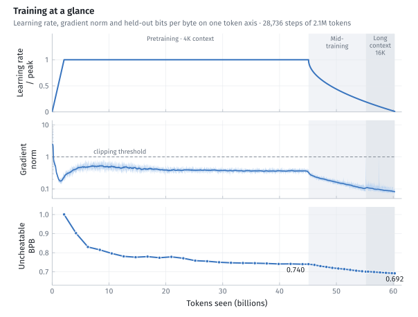
Figure 10: LR schedule, gradient norm and UncheatableEval bpb with tokens seen.

From Figure 10, we can see that the gradients behave well, and the UncheatableEval bpb decreases monotonically.

Performance analysis

To evaluate the model, we compare against some well-known open-source competitors in the same class. We evaluate the model on standard pretraining benchmarks as well as the July 2026 UncheatableEval data, published after every model's training cut-off. We also provide accuracy vs FLOPs/token and training compute plots.

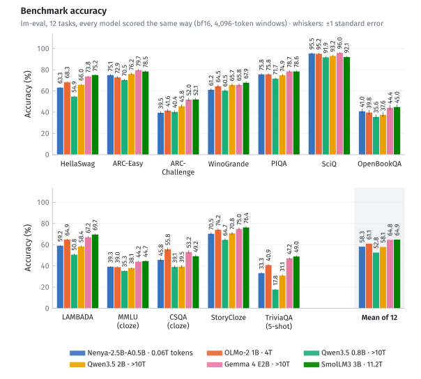
Figure 11: Pretraining benchmarks computed with lm-eval. Methodology described on our HF page. Training data was decontaminated against the 14 benchmark evaluation sets.

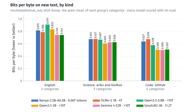
Figure 12: Bits per byte on the July 2026 UncheatableEval dataset, split by category.

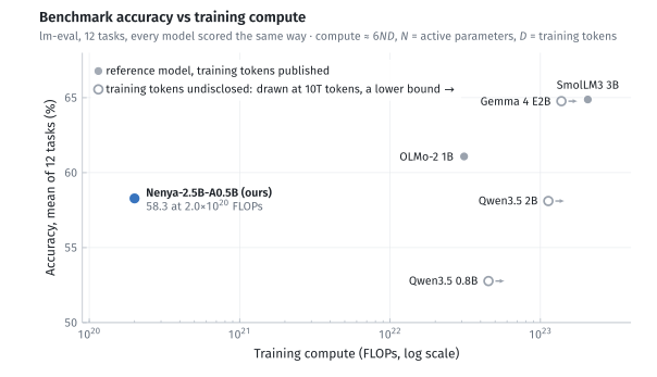
Figure 13: Accuracy (lm-eval, mean of 12 tasks) against estimated training compute $6ND$ ($N$ active parameters, $D$ training tokens). Nenya reaches 58.3 with 2.0×10²⁰ FLOPs, 155× less than OLMo-2 1B (61.1). Qwen3.5 and Gemma 4 do not publish their token counts: they are drawn at 10T tokens, a lower bound (hollow markers).

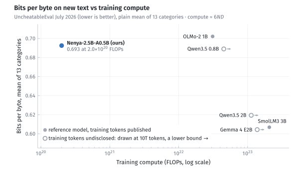
Figure 14: UncheatableEval bits per byte on text published in July 2026, after every model here was trained (plain mean of 13 categories, lower is better), against estimated training compute.

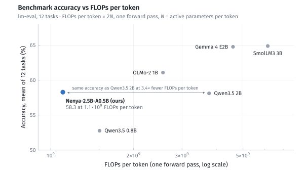
Figure 15: Accuracy against active FLOPs per token: one forward pass, 2 × active parameters, the cost of running the model. Nenya matches Qwen3.5 2B (58.3 vs 58.1) at 3.4× fewer FLOPs per token: 1.1×10⁹ vs 3.8×10⁹.

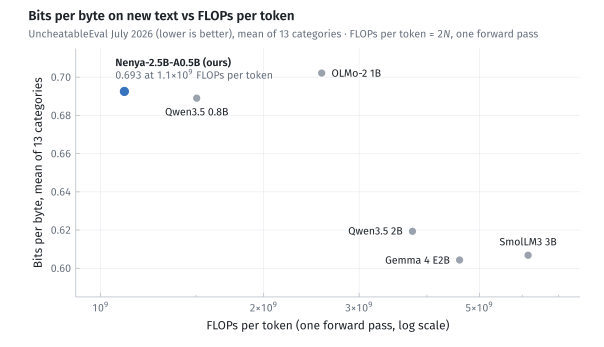
Figure 16: UncheatableEval July 2026 bits per byte against active FLOPs per token (one forward pass).

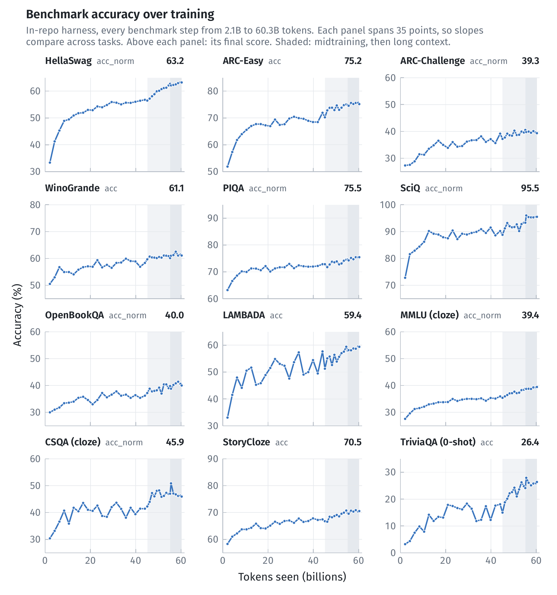
Figure 17: How individual tasks improve with tokens.

Figures 11 and 12 show that our model is competitive with Qwen3.5 2B, better than Qwen3.5 0.8B, but worse than Gemma 4 E2B, SmolLM3 3B and slightly worse than OLMo-2 1B on the standard pretraining benchmarks. As older validation sets have a possibility of being in the training data (though we explicitly decontaminate), we also show the UncheatableEval July 2026 bits per byte over three categories, on text published after every model's training cut-off. From this, we can see that Nenya does well on English, beating Qwen3.5 2B, but trails it by 11% on science and does worst on code. Nenya's UncheatableEval results can be partly explained by our training data distribution, which contains only 10% code and mostly web data.

From Figures 13–16, we can see that Nenya is an efficient learner, rivalling the likes of Qwen3.5 2B with ~500× lower training compute. For models that do not disclose their training token count, we assume 10T; however, it's likely 30T+ as that is what their last generations were trained on. What is more interesting for on-device agents is that it rivals Qwen3.5 2B with 3.4× fewer active FLOPs/token.

Figure 17 demonstrates how benchmark performance improves with token count. We can see that most tasks are still improving rapidly while PIQA and SciQ have saturated.

Optimised Mac implementation

A clear benefit of Nenya is its accuracy per active parameter. To materialise this, we provide v1 of our optimised Mac implementation. It can be installed through our pip package.

pip install "nenya[mac]"

import nenya
print(nenya.generate("The mitochondrion is the organelle responsible for", max_new_tokens=40))
print(nenya.generate("Question: What is the capital of Australia?\nAnswer:", max_new_tokens=8, temperature=0))

This section highlights the results on M1 (oldest) and M4 (newest-ish) Macs, and provides an overview of the optimisations made.

	Apple M4 (base)	Apple M1 (base)
Model	Nenya-2.5B-A0.5B (the release)	Nenya-2.5B-A0.5B (the release)
Engine weight file	3.47 GB	3.47 GB
Decoding speed (tokens/s)
Empty context	127.1	74.3
1K tokens	123.9	72.5
4K tokens	114.1	67.6
16K tokens	92.5	55.5
Peak memory while decoding
At 1K tokens	4.10 GB	4.07 GB
At 16K tokens	4.30 GB	4.26 GB
Without the weight file (1K / 16K)	0.67 / 0.86 GB	0.54 / 0.73 GB

Prompt processing and time to first token on the Apple M4:

Prompt length (tokens)	16	64	256	1,024	4,096	16,384
Time to first token (s)	0.04	0.06	0.15	0.57	2.7	18.6
Prompt processing (tokens/s)	392	1,129	1,720	1,801	1,510	909

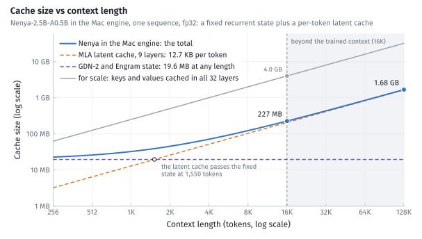
Figure 18: How total cache size varies with context size and its constituents. Note the cache is in fp32.

Figure 18 shows how the total cache size, and each of its parts, grows with context length. Note that the KV cache is still unoptimised in this release.

The Metal engine is Objective-C++ host code plus custom Metal GPU kernels. We found PyTorch (MPS backend) and MLX slower. We also found using the NPU slower for the following reasons:

• It doesn't support the routing, hashing and recurrent state requirements of our model, adding processor-switching overheads.
• On the roofline model, we are memory-bandwidth-bound, and the NPU and GPU share the same memory bandwidth.

For the Metal engine, we make the following optimisations:

• Weights are stored and loaded in 8-bit with per-group scales and converted to fp16 after load to reduce memory bandwidth. The MoE router stays in fp32, as we found lower-precision routers did not reproduce the expert selection seen in training.

• The LM head is the biggest cost per step, so we take a multi-pass approach: we score every vocabulary row with 4-bit weights and, after a selection step, rescore a subset in fp16. This enables fp16 precision at 4-bit cost.

• Where possible, we merge and store matrices that act on one input together. For example, for the seven Gated DeltaNet-2 projections, $q$, $k$, $v$, $b$, $w$, $f$ and $g$ are stored and computed as one kernel call, to avoid kernel launch overheads.

• We keep all the work on the GPU to avoid processor-switching costs (GPU <-> NPU <-> CPU), and token-reading work on the CPU is pipelined with GPU processing.

• We fuse each major operation into a single kernel to avoid kernel launch overheads. The convolution, gates, decay, normalisation, recurrence and gated norm of GDN-2 are one kernel; Engram hashing and table lookup are one kernel; and each mHC boundary is one kernel. At the start of optimisation, we found kernel launch overhead to be the biggest issue.

• mHC between two sublayers computes 24 control parameters: 4 for the read, 4 for the write and 16 for the mixing matrix. The following sublayer is blocked until these can be computed, which takes about 25 µs on the critical path but happens 64 times per token. We use the linearity of the mHC computation to unblock the next sublayer computation, reducing the 25 µs to 10 µs.

• For long context, we use a FlashMLA-style attention kernel with 64-row tiles, a running softmax and each cache value read once per phase.

There are several optimisations still to be made in quantisation, Engram memory layout, mHC orthogonalisation, arithmetic operations and the KV cache, but we defer those to v2 of the engine.

Pretraining data mix

Figure 19 shows the dataset category composition we used for training.

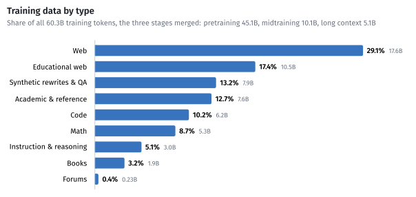
Figure 19: Dataset category composition.

Packing: For each source, we join the documents into a long token stream, separated by EOT tokens. We cut this stream into 4,096-token rows. Each mini-batch takes rows from different categories of our training data so we maintain the mix shown in Figure 19. We also shuffle each mini-batch. We call this source packing. For instruction data, we want each question/answer pair inside one 4,096-token row, so we pack whole Q/A pairs and pad any leftover token slots instead of cutting a pair.

Document masking: Training rows can hold multiple documents in the same 4,096-token training window, so we apply document masking to stop the model looking across the boundaries and polluting the context. The EOT token decides the document boundaries. For MLA, we apply block-diagonal masking to limit the keys each query attends to, using varlen kernels from FlashAttention. For Gated DeltaNet-2, we reset the recurrent state at the EOT token and for Engram, we stop the n-gram hashes at the document boundary and limit the convolutions too.

Decontamination: We match the questions and answers from the 14 benchmark evaluation sets against the training data. We take 13-word and 8-word windows of text, normalise them and hash them to compare against training data windows, and if we see benchmarks matching the training data, we cut out the matching span plus 200 characters either side. Documents with more than 5 matches, and synthetic, instruction and code documents, are dropped whole, as cutting would leave broken examples unfit for training.

Deduplication: We keep one dedup index per training stage, shared by every source, which every document is checked against. We key documents with a 128-bit hash, and drop every subsequent copy where the hash matches. Web sources are deduped by their normalised URL so the same page formatted differently doesn't sneak in. In total, we remove 7.6–9.3% of documents per stage as exact duplicates, almost all of them Stack-Edu files that our source data stores several times.

Model configuration

Nenya has the following configuration.

ARCHITECTURE DETAILS
Total Parameters	2.59B
Activated Parameters	553M
Routed-Expert Parameters	1.59B (6 of 120 experts run per token)
Engram Table Parameters	528M
Number of Layers	32
Number of Dense Layers	2 (blocks 0 and 1)
Attention-Layer Composition	23 Gated DeltaNet-2 (GDN-2) + 9 Multi-head Latent Attention (MLA), the MLA at blocks 0, 3, 7, 11, 15, 19, 23, 27, 31
Attention Hidden Dimension ($d_{model}$)	960
Number of Attention Heads	12 (for both attention types)
MLA	Normalised 320-dim key/value latent plus a 32-dim key shared by all heads
GDN-2	Head Dimension 128
Dense FFN Hidden Dimension	2,560 (SwiGLU)
Latent MoE Dimension	384
MoE Hidden Dimension (per Expert)	384
Number of Experts	120
Selected Experts per Token	6
Number of Shared Experts	2
MoE Balancing	Quantile Balanced
Engram Memory	Before blocks 1 and 14; 8 hash heads per order
Residual Streams	4
Vocabulary Size	100,278
Padding Rows	74
Context Length	16,384
Attention Mechanism	GDN-2 & MLA
Activation Function	SwiGLU
Precision	bf16
Modality	Text
Positional Encoding	None

Summary and reflections

Is Nenya interesting? mHC, Engram and MoE are acting synergistically to do something interesting, and the ability to rival larger models with significantly lower training compute and FLOPs/token should not go unnoticed. We could argue that most benchmark gains come early and training for another 10T tokens won't help, but the benchmark vs token trajectories of OLMoE, TinyLlama and Pythia show that it is not true. It also wouldn't explain the competitive bpb on unseen text.

For future models, there are clear issues we aim to solve:

• Training warmup was a little longer than necessary; we could get away with 250 steps as the model is generally quite stable.

• A context size of 16K works for many use cases, but for long running agents, 128K+ would be ideal.

• The placement of the block 14 Engram should be optimised, or its parameters allocated elsewhere.

• We should have added an RMSNorm after each FFN to control the scale of its output.

• We have not yet computed scaling laws for this architecture.

Appendix

A1. How stream spread is calculated (Figure 4a)

For each of the $N=\mathrm{8,192}$ validation tokens, let $x_{t,1},\dots ,x_{t,4}\in {\mathbb{R}}^{960}$ be the four streams leaving the last block (block 31), and ${\overline{x}}_t$ their mean:

$${\overline{x}}_t=\frac{1}{4}\sum _{k=1}^4{x}_{t,k},\text{spread}=\frac{{\displaystyle \frac{1}{4N}}{\displaystyle \sum _{t=1}^N\sum _{k=1}^4\Vert x_{t,k}-{\overline{x}}_t{\Vert }_2}}{{\displaystyle \frac{1}{N}}{\displaystyle \sum _{t=1}^N\Vert {\overline{x}}_t{\Vert }_2}}$$

A spread of 0 means the four streams are identical.

A2. How the read and write shares are computed (Figure 5)

For every token $t$ of 8 fixed validation sequences ($N=\mathrm{8,192}$ tokens), each sublayer's mHC module computes a read weight and a write weight for each of the four streams $k$:

$$H_{t,k}^{\text{pre}}\in (0,1),H_{t,k}^{\text{post}}\in (0,2)$$

The read weights set how much of each stream goes into the mix the sublayer reads; the write weights set how much of its output is added to each stream. Both are averaged over tokens, and each stream's average is divided by the sum over the four streams:

$${\text{read share}}_k=\frac{{\overline{H}}_k^{\text{pre}}}{\sum _{j=1}^4{\overline{H}}_j^{\text{pre}}},{\text{write share}}_k=\frac{{\overline{H}}_k^{\text{post}}}{\sum _{j=1}^4{\overline{H}}_j^{\text{post}}},{\overline{H}}_k=\frac{1}{N}\sum _{t=1}^N{H}_{t,k}$$

Each sublayer's four shares add up to 1. A write share is exactly the fraction of the sublayer's output that lands in stream $k$, since the same output goes to every stream. A read share is the stream's weight in the mix, which is RMS-normalised before the sublayer uses it, so only these ratios matter. Values are from the final checkpoint.

A3. Mixing-matrix diagonal (Figure 6)

For every token $t$, each sublayer's mHC module mixes the four streams with a $4\times 4$ matrix $H_t^{\text{res}}$ whose rows sum to 1, so each new stream is a weighted average of the four. Figure 6 shows its diagonal, averaged over the four streams and the $N=\mathrm{8,192}$ validation tokens:

$$\text{diagonal}=\frac{1}{4N}\sum _{t=1}^N\sum _{k=1}^4{H}_{t,kk}^{\text{res}}$$

The identity matrix, which leaves the streams unmixed, gives 1; the uniform matrix, which replaces every stream with the average of all four, gives 0.25.

A4. Memory size relative to the streams (Figure 7b)

For one Engram layer, let $x_{t,k}\in {\mathbb{R}}^{960}$ be stream $k$ entering the layer for token $t$, and $y_{t,k}$ what the layer adds to it, over the $N=\mathrm{8,192}$ validation tokens. Figure 7b shows the ratio of their sizes over all tokens and streams:

$$\text{ratio}=\sqrt{\frac{\sum _{t=1}^N\sum _{k=1}^4\Vert y_{t,k}{\Vert }_2^2}{\sum _{t=1}^N\sum _{k=1}^4\Vert x_{t,k}{\Vert }_2^2}}$$

A ratio of 0.38 means the memory adds 38% of the streams' size.

A5. Table row norm (Figure 7d)

For each token, each Engram layer reads one 60-value row from each of its 16 hash tables (8 bigram and 8 trigram), 960 values in total. Figure 7d shows the mean L2 norm of the $R$ rows the optimiser has updated so far, which from step 500 on is every row:

$$\overline{\Vert E\Vert }=\frac{1}{R}\sum _{r=1}^R\Vert E_r{\Vert }_2,E_r\in {\mathbb{R}}^{60}$$

A6. Routed share (Figure 8a)

For one MoE block, let $r_t\in {\mathbb{R}}^{960}$ be the routed experts' output for token $t$ (the weighted sum of its 6 experts, after the up-projection) and $s_t$ the shared experts' output, over the $N=\mathrm{8,192}$ validation tokens. The block's output is $r_t+s_t$, and the routed share is the routed part's projection onto it:

$$\text{routed share}=\frac{\sum _{t=1}^N⟨r_t,r_t+s_t⟩}{\sum _{t=1}^N\Vert r_t+s_t{\Vert }_2^2},\text{shared share}=1-\text{routed share}$$

A7. Expert load (Figure 8b)

An optimiser step trains on $T=\mathrm{2,097,152}$ tokens, each sent to 6 of the 120 experts, so every MoE block fills $6T$ token slots. Expert $e$ of block $l$ receives $c_{l,e}$ of them, against a fair share of $6T/120$, 1/120 of the slots. Figure 8b shows each block's busiest and least-used expert relative to that, averaged over the 30 MoE blocks:

$$\text{busiest}=\frac{1}{30}\sum _{l=1}^{30}\underset{e}{max}\frac{c_{l,e}}{6T/120},\text{least used}=\frac{1}{30}\sum _{l=1}^{30}\underset{e}{min}\frac{c_{l,e}}{6T/120}$$

The 1.43× and 0.75× quoted for pretraining are the medians over its evals.

A8. Routing entropy (Figure 8c)

With $c_{l,e}$ the token slots expert $e$ of block $l$ receives in one optimiser step (Appendix A7), each expert's share is $f_{l,e}=c_{l,e}/6T$. Figure 8c shows the entropy of these shares, divided by its maximum, $\log 120$, and averaged over the 30 MoE blocks:

$$H=\frac{1}{30}\sum _{l=1}^{30}\frac{-\sum _{e=1}^{120}{f}_{l,e}\log f_{l,e}}{\log 120}$$

$H=1$ when every expert receives the same number of slots, and ${120}^H$ is the number of equally used experts with the same entropy. The line is the median of every 16 steps and the band their range.

A9. Routed experts in effect (Figure 8e)

Token $t$ is sent to 6 experts with weights $p_{t,1},\dots ,p_{t,6}$, a softmax over their router scores, so $\sum _{i=1}^6{p}_{t,i}=1$. The number of experts in effect is

$$k_{\text{eff}}=\frac{1}{N}\sum _{t=1}^N\frac{1}{\sum _{i=1}^6{p}_{t,i}^2}$$

which is 6 when the weights are equal and 1 when one expert takes all the weight. The plot shows its mean over the last 10 evals.

A10. Expert specialisation (Figure 9)

The final checkpoint is run on 640 rows of 1,024 tokens of UncheatableEval July 2026, a third each English, science and code. For each routed expert $e$ of every MoE block, $c_{e,k}$ counts the tokens of kind $k$ that pick it among their 6, and $n_k$ is the number of tokens of that kind. Its mix of kinds is its pick rate per token, normalised to sum to 1:

$$m_{e,k}=\frac{c_{e,k}/n_k}{\sum _{j=1}^3{c}_{e,j}/n_j}$$

Each of the 3,600 routed experts (120 in each of the 30 MoE blocks) is a dot at $(m_{e,1},m_{e,2},m_{e,3})$: an expert picked equally often on all three kinds sits in the centre, a pure specialist in a corner. It is coloured when one kind makes up more than half of its mix.

A11. FLOPs per token and training compute (Figures 13–16)

$N$ is a model's active parameters: the weights one token's forward pass multiplies by. Lookups cost no multiplications and are left out (our Engram tables, untied input embeddings, Gemma's per-layer embeddings), as are vision and audio encoders and multi-token-prediction heads; a tied embedding counts once, as the output head. For Nenya, that is 2,594.7M stored parameters minus the 528.5M in the Engram tables and the 1,512.9M in the 114 of 120 routed experts per block that a token does not use, giving a final 553.3M.

A forward pass costs one multiply and one add per active weight, and the backward pass about twice that, so with $D$ training tokens:

$$\text{FLOPs per token}=2N,\text{training compute}=6ND$$

Attention-score FLOPs, which grow with context, are left out for every model; at 4K context they would add about 10% for the dense models and a few percent for the hybrids. Qwen3.5 and Gemma 4 do not publish $D$, so they are drawn at 10T tokens, a lower bound. Appendix A12 lists each model's $N$, $D$ and training compute.

A12. Benchmark tables

Active parameters are the weights each token is multiplied by, as used for the compute estimates in Figures 13–16; total parameters are all stored weights. Training FLOPs are $6ND$.

Model	Training tokens	Active parameters	Total parameters	Training FLOPs
Nenya	0.06T	0.55B	2.59B	2.0 × 10²⁰
OLMo-2 1B	4.05T	1.28B	1.48B	3.1 × 10²²
Qwen3.5 0.8B	>10T (est.)	0.75B	0.87B	≥ 4.5 × 10²²
Qwen3.5 2B	>10T (est.)	1.88B	2.27B	≥ 1.1 × 10²³
Gemma 4 E2B	>10T (est.)	2.30B	5.12B	≥ 1.4 × 10²³
SmolLM3 3B	11.2T	3.08B	3.08B	2.1 × 10²³

On the standard pretraining benchmarks, the model achieves the following. Accuracies are in %, ± one standard error.

lm-eval task	Metric	Nenya (0.06T tokens)	OLMo-2 1B (4T tokens)	Qwen3.5 0.8B (>10T tokens)	Qwen3.5 2B (>10T tokens)	Gemma 4 E2B (>10T tokens)	SmolLM3 3B (11.2T tokens)
hellaswag	acc_norm	63.3 ± 0.5	68.3 ± 0.5	54.9 ± 0.5	66.0 ± 0.5	73.8 ± 0.4	75.2 ± 0.4
arc_easy	acc	75.1 ± 0.9	72.9 ± 0.9	70.5 ± 0.9	76.2 ± 0.9	79.7 ± 0.8	78.5 ± 0.8
arc_challenge	acc_norm	39.5 ± 1.4	41.6 ± 1.4	40.4 ± 1.4	45.8 ± 1.5	52.0 ± 1.5	52.1 ± 1.5
winogrande	acc	61.2 ± 1.4	64.5 ± 1.3	60.5 ± 1.4	65.7 ± 1.3	65.8 ± 1.3	67.9 ± 1.3
piqa	acc_norm	75.8 ± 1.0	75.8 ± 1.0	71.7 ± 1.1	74.9 ± 1.0	78.7 ± 1.0	78.6 ± 1.0
sciq	acc_norm	95.5 ± 0.7	95.2 ± 0.7	91.9 ± 0.9	93.2 ± 0.8	96.0 ± 0.6	92.1 ± 0.9
openbookqa	acc_norm	41.0 ± 2.2	39.8 ± 2.2	35.6 ± 2.1	37.6 ± 2.2	44.4 ± 2.2	45.0 ± 2.2
lambada_openai	acc	59.2 ± 0.7	64.9 ± 0.7	50.8 ± 0.7	58.4 ± 0.7	67.2 ± 0.7	69.7 ± 0.6
mmlu_cloze	acc_norm	39.3 ± 0.4	39.0 ± 0.4	35.3 ± 0.4	38.1 ± 0.4	44.2 ± 0.4	44.7 ± 0.4
csqa_cloze	acc_norm	45.8 ± 1.4	55.8 ± 1.4	39.1 ± 1.4	39.5 ± 1.4	53.2 ± 1.4	49.2 ± 1.4
xstorycloze_en	acc	70.5 ± 1.2	74.2 ± 1.1	64.7 ± 1.2	70.8 ± 1.2	75.0 ± 1.1	76.4 ± 1.1
triviaqa_5shot_greedy	acc	33.3 ± 0.7	40.9 ± 0.8	17.8 ± 0.6	31.1 ± 0.7	47.2 ± 0.8	49.0 ± 0.8
avg	mean of all	58.3	61.1	52.8	58.1	64.8	64.9

On UncheatableEval (July 2026), grouped by category, the model scores the following bits per byte (lower is better).

Group	Nenya (0.06T tokens)	OLMo-2 1B (4T tokens)	Qwen3.5 0.8B (>10T tokens)	Qwen3.5 2B (>10T tokens)	Gemma 4 E2B (>10T tokens)	SmolLM3 3B (11.2T tokens)
English (3 categories)	0.815	0.788	0.911	0.833	0.745	0.741
Science: arXiv and bioRxiv (5 categories)	0.674	0.677	0.667	0.605	0.624	0.626
Code: GitHub (5 categories)	0.637	0.676	0.578	0.505	0.500	0.507

A13. GDN-2 inner workings

After the mHC read from the residual stream converts the 4-stream hidden state into a single stream, $x_t$, we project it into keys, values and queries, just as in standard attention, as well as decay, erase, write and output gates to give the network attenuation control over incoming and outgoing values.

Inputs

Our head dimension is $d_{head}=128$. The query, key and value are each mixed with the previous 3 tokens by a short causal convolution; the query and key are then scaled to unit length so updates don't wash out existing information in $S$.

$$\begin{array}{}\text{(}\text{1}\text{)}& q_t,k_t,v_t=\mathrm{SiLU}(\mathrm{Conv}1\mathrm{d}(W_q{x}_t)),\dots q_t,k_t\leftarrow \frac{q_t}{\Vert q_t\Vert },\frac{k_t}{\Vert k_t\Vert }\end{array}$$

Gates

The decay gate, $g$, has one value per key channel, which depends on the token, and is scaled by $e^{A_h}$, where $A_h$ is an nn.Parameter learned for each head that does not depend on the token. We use a negative exponential to contain the value between 0 and 1 as it's a decay gate:

$$\begin{array}{}\text{(}\text{2}\text{)}& g_t=-e^{A_h}\mathrm{softplus}(W_f{x}_t+b_f)\in (-\mathrm{\infty },0{]}^{d_{head}}\end{array}$$

The erase gate, $b$, controls how strongly each key channel removes what is already stored under the current key.

$$\begin{array}{}\text{(}\text{3}\text{)}& b_t=\sigma (W_b{x}_t)\in (0,1{)}^{d_{head}}\end{array}$$

The write gate, $w$, controls how much of each value channel is stored.

$$\begin{array}{}\text{(}\text{4}\text{)}& w_t=\sigma (W_w{x}_t)\in (0,1{)}^{d_{head}}\end{array}$$

State update ($S_t\in {\mathbb{R}}^{d_{head}\times d_{head}}$, keys × values)

Decay first:

$$\begin{array}{}\text{(}\text{5}\text{)}& S^{\prime }=\mathrm{Diag}(e^{g_t})S_{t-1}\end{array}$$

Each key row of the memory fades at its own rate, set by the decay gate $g_t\le 0$.

Delta update:

$$\begin{array}{}\text{(}\text{6}\text{)}& S_t=S^{\prime }+k_t(w_t\odot v_t-S^{\prime \mathrm{\top }}(b_t\odot k_t){)}^{\mathrm{\top }}\end{array}$$

Erase what the key $k_t$ already retrieves from the faded memory, then write the new value.

• $S^{\prime \mathrm{\top }}(b_t\odot k_t)$: what the faded memory currently returns for this key, with each key channel weighted by the erase gate $b_t$.
• $w_t\odot v_t$: the new value, with each value channel weighted by the write gate $w_t$.
• $w_t\odot v_t-S^{\prime \mathrm{\top }}(b_t\odot k_t)$: the correction, the new value minus what is already stored.
• $k_t(\cdots {)}^{\mathrm{\top }}$: adds that correction to the memory under the current key, leaving entries for other keys untouched.

Read and output projection

$$\begin{array}{}\text{(}\text{7}\text{)}& o_t=\frac{S_t^{\mathrm{\top }}{q}_t}{\sqrt{d_{head}}}\end{array}$$

Looks up the memory with the query: a weighted mix of the values whose keys are similar to $q_t$.

$$\begin{array}{}\text{(}\text{8}\text{)}& y_t=W_o[\mathrm{RMSNorm}(o_t)\odot \sigma (W_g{x}_t)]\end{array}$$

Normalises each head's output, gates it per channel by the token, and projects it back to the model width.