Quantile balancing

For MoE architectures, a key concern is experts vanishing and becoming redundant, resulting in wasted FLOPs and memory while hurting performance. In an ideal case, experts would be at 100% utilisation and specialise in different domains or aspects of language modelling. Recent latent fine-grained MoE architectures scaled up experts to ~900 (Kimi K3). A key reason for this is quantile balancing, a loss-free method introduced and used for expert balancing.

MoE overview

Rather than having a fixed feed-forward layer in our model, what if we could have many and cleverly route each token? It would give us more capacity without increased FLOPs. That is what MoEs try to achieve and the key component in a MoE architecture is the router. It's a learned linear projection that takes as input the token vector and outputs a vector of length equal to the number of experts, which represents the expert scores; we refer to these as the logits. If we route each token to three experts (top-3), we use the index positions of the top three logits to route the token to. For example, if the 10th, 113th and 89th index positions of the assignment vector have the largest values, these are the three experts we route to. The token is then multiplied by the weight matrices of each selected expert and the output from each is scaled by the softmax of the logits (to bake in how much contribution we want from each expert) and summed. The training signal to the router comes from the softmax-weight multiplication, not the assignments, as that is a non-differentiable operation.

Say we have $x \in R^{b \times t \times d_{m o d e l}}$ , where $b$ is the batch size, $t$ is the number of tokens and $d_{m o d e l}$ is our internal model dimension of our hidden states and embeddings. We pass it through our router projection to get our assignment scores:

\begin{matrix} (1) & s = x W_{router} \end{matrix}

where $s \in R^{b \times t \times n u m_e x p e r t s}$ and $n u m_e x p e r t s$ is the number of experts we have. To make our router selection from $s$ , we can simply do

\begin{matrix} (2) & topk_scores, topk_indices = topk (s, k = 3) \end{matrix}

to select the index positions of the top three highest scores, as well as the scores themselves.

In code, it's implemented as follows:

# Defining a linear layer
router = nn.Linear(cfg["d_model"], cfg["num_experts"], bias=False)

# Logit scores
# x is our model's hidden state
# [b, t, d_model] -> [b, t, num_experts]
scores = router(x)

# torch.topk returns the top k values and
# their indices
topk_scores, topk_indices = torch.topk(scores, k=3)

# Softmax the top k logits 
# to get probs to scale outputs with
topk_probs = torch.softmax(topk_scores, dim=-1)

How the tokens get routed efficiently is outside the scope of this post.

Mechanics of router collapse

A router collapse is a situation where tokens are being excessively assigned to a small subset of experts. This in turn means that the unselected ones do not get trained and linger around as dead parameters. It is also a self-reinforcing cycle as the router starts to prefer the excessively assigned experts as they are more trained, ensuring the expert concentration grows stronger with training.

Looking at the mechanistic cause, when a token is multiplied by the router projection, if some columns in the router weights have a significantly larger magnitude than the rest, then these router positions will be picked for all tokens, assuming the magnitude of the token vector itself isn't super small and the resulting dot product with the token vector is large.

Remedies

Several methods have been tried, starting with load-balancing losses, then bias additions and, finally, the subject of this post, quantile balancing.

Auxiliary loss-free bias balancing

Bias balancing is a simple but clever approach introduced by DeepSeek-V3. It looks at the state of current routing, and adds a small value to help underloaded experts and deter overloaded experts.

Suppose you have 4 experts, 4 tokens and top- $k$ routing with $k = 1$ , and the following token assignments produced by the router:

Token	E1	E2	E3	E4	Selected
t1	0.90	0.75	0.70	0.50	E1
t2	0.70	0.85	0.80	0.70	E2
t3	0.55	0.60	0.85	0.80	E3
t4	0.65	0.65	0.90	0.60	E3

Table 1: Token assignments.

A uniform spread would be the number of tokens divided by the number of experts, giving us 1 token per expert, but from the above, we can see that expert 1 gets 1 assignment, expert 2 gets 1, expert 3 gets 2 and expert 4 gets none, creating an imbalance.

Given that we can count the degree of imbalance, simply by looking at the difference between ideal and actual, and we know what the ideal balance should be, we can nudge the router scores towards a more even selection. We call this nudge a bias and it's computed as:

\begin{matrix} (3) & \begin{aligned} β_{n e w} & = β_{o l d} + λ sign (c_{i d e a l} - c_{a c t u a l}) \\ sign (z) & = {\begin{cases} 0 & if z = 0 \\ 1 & if z > 0 \\ - 1 & if z < 0 \end{cases} \end{aligned} \end{matrix}

where $λ$ controls how strongly we want to update the bias term, $β_{n e w}$ and $β_{o l d}$ (zero at step 0 in training) are the new and old biases, $c_{i d e a l}$ is $\frac{t \cdot k}{n u m_e x p e r t s}$ , the ideal allocation, and $c_{a c t u a l}$ is the actual allocation.

To correct the imbalance, when it comes to selecting our experts in the next training iteration, we now do the following for Eq. 2:

\begin{matrix} (4) & topk (s + β, k = 3) \end{matrix}

Where $β$ is a $n u m_e x p e r t s$ -dimensional vector, and the same vector is added to each token. There is no impact on the weights of the router or the model, and we call .detach() on the bias (in some sense, it does blindside the model). We compute the biases in one batch but apply them to the next to preserve causality. This counters any global concentration trends over the course of training.

For the example in Table 1, our $c_{a c t u a l} = [1, 1, 2, 0]$ while $c_{i d e a l} = [1, 1, 1, 1]$ . We can calculate the new biases and we'll assume the old biases are zero. We'll make $λ = 0.05$ and $k = 1$ and get the following biases:

\begin{matrix} (5) & \begin{aligned} β_{E 1} & = 0.05 sign (1 - 1) = 0 \\ β_{E 2} & = 0.05 sign (1 - 1) = 0 \\ β_{E 3} & = 0.05 sign (1 - 2) = - 0.05 \\ β_{E 4} & = 0.05 sign (1 - 0) = + 0.05 \end{aligned} \end{matrix}

Now if we add these to our assignments from Table 1, we get:

Token	E1 + 0	E2 + 0	E3 − 0.05	E4 + 0.05	Selected
t1	0.90	0.75	0.65	0.55	E1
t2	0.70	0.85	0.75	0.75	E2
t3	0.55	0.60	0.80	0.85	E4
t4	0.65	0.65	0.85	0.65	E3

Table 2: Assignments after the bias addition.

All experts now have 1 token each, as one token switches from E3 to E4.

An issue with bias balancing is that though the direction of the update is computed from the data, the size of the update, $λ$ , is a hyperparameter and has to be ablated, which adds extra time and costs. Getting it wrong is also costly, as it can lead to imbalance, the very artefact it's designed to solve.

Quantile balancing

Quantile balancing works just like bias balancing, but it goes further to compute the magnitude of the bias from expert assignment vectors, not just the sign.

It asks the following question: For each expert, how far was it from being selected in the top-k for each token, and what values would I need to add to this expert so it can have its fair share?

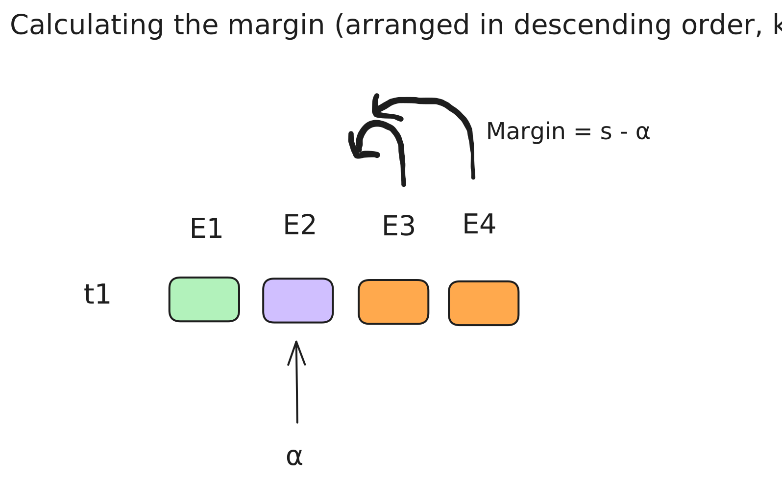
This means we need a distance from selection per token, per expert. We call this distance the margin, $m$ . We begin by understanding what logit each expert would have needed to make the assignment threshold for its token. This would be the difference between the current assignment score $s$ and the cut-off value, which we refer to as $α$ . If we sorted our assignment vector in descending order, and travelled from left to right, $α$ would be the first value of an unassigned expert. Everything to the left of it would be an expert that was assigned the token, and everything to the right of it was unassigned.

margins

Figure 1: Calculating the cut-off and margin. Green is the assigned expert; orange and purple are the unassigned experts.

\begin{matrix} (6) & m_{i, j} = s_{i, j} - α_{i} \end{matrix}

Where $m_{i, j}$ is the margin of the $j$ -th expert for the $i$ -th token, $α_{i}$ is the cut-off for the $i$ -th token and $s_{i, j}$ is the assignment score for the $j$ -th expert of the $i$ -th token. In order to answer our question, we want a vector per expert, that tells us how far it was from making each token, so after we calculate the margins, we organise them per expert. This will give us $n u m_e x p e r t s$ vectors of size $t$ . Figure 2 shows how this would look.

margin_vectors

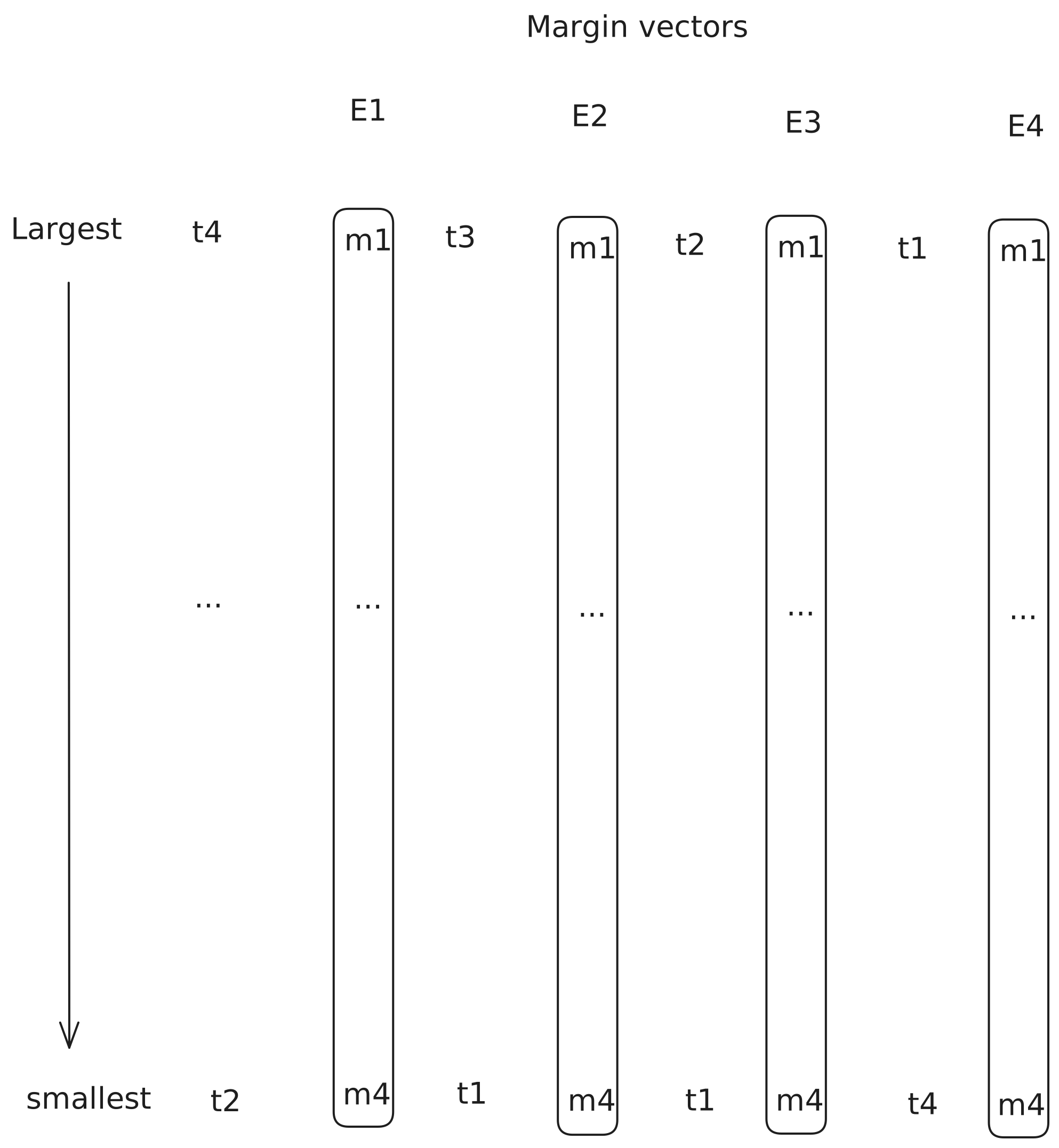
Figure 2: Margin vectors for our experts.

For each expert's margin vector, we would have positive values and negative values. The positives would be where it was selected for that token and the negatives would be where it missed out by the margin amount. The point at which the values cross from positive to negative is known as the pivot point. Figure 3 shows how to interpret the margin vector.

ideal_vs_current_pivot

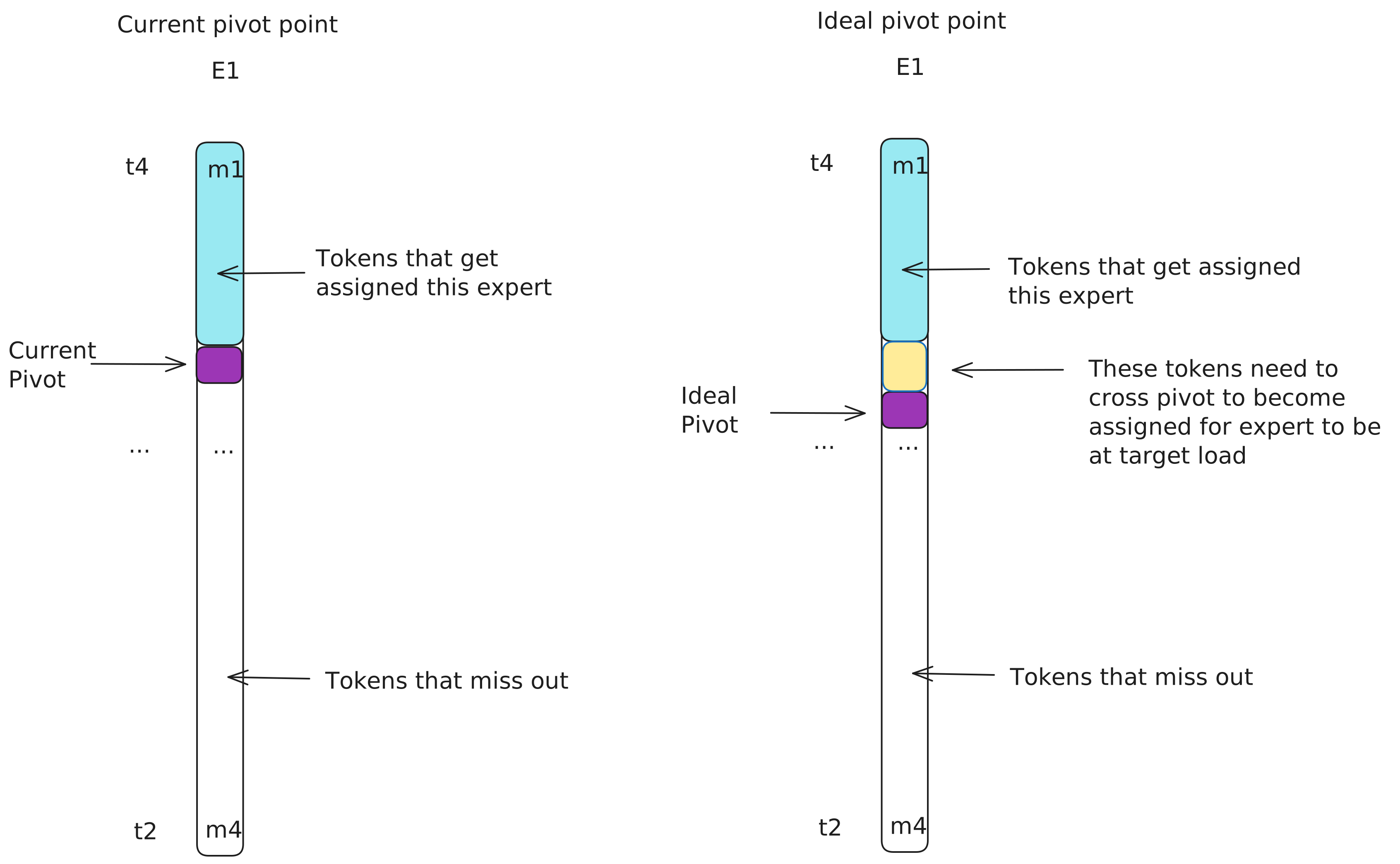
Figure 3: Changing the pivot point of the margin vector helps us balance this expert.

We have now answered the first part of our question, and we can move on to the second, what value would I need to add for each expert to get its fair share. Given 4 experts and 4 tokens with $k = 1$ , the target load is:

\begin{matrix} (7) & q = \frac{t \times k}{n u m_e x p e r t s} = \frac{4 \times 1}{4} = 1 \end{matrix}

So each expert needs 1 token, which is 25% of the tokens, and turning that into a percentile is:

\begin{matrix} (8) & p = 1 - \frac{k}{n u m_e x p e r t s} = 1 - \frac{1}{4} = 0.75 \end{matrix}

So for each expert, we would want to have the ideal pivot point at the 75th percentile. As we can see from Figure 3, we have an initial pivot point for our unbalanced expert and we would like a new pivot point which leads to a balanced expert. This point is:

\begin{matrix} (9) & β_{j} = - Q_{0.75} (m_{:, j}) \end{matrix}

where $Q_{0.75}$ is the 75th percentile over the tokens, and this is our bias. Intuitively, this will move 25% of the margin values positive and above the pivot, meaning the expert would be assigned those tokens; the pivot moves to zero, and the other 75% fall below it and stay unassigned. This would mean our expert is well balanced.

We do this for each expert to get four bias values, one per expert. We can then add these to each token in the next batch to help balance allocations.

\begin{matrix} (10) & topk (s + β, k = 3) \end{matrix}

Unlike loss-free bias balancing, we do not compute an update to the biases, but new total biases. To continue the numerical example from Table 1, we have

Token	E1	E2	E3	E4	$α$
t1	0.90	0.75	0.70	0.50	0.75
t2	0.70	0.85	0.80	0.70	0.80
t3	0.55	0.60	0.85	0.80	0.80
t4	0.65	0.65	0.90	0.60	0.65

Table 3: Cut-off value per assignment vector.

Where the $α$ column is the cut-off value per assignment vector. For each assignment vector, we subtract this cut-off value from each expert assignment value to get the following margin vectors:

Token	E1	E2	E3	E4
t1	+0.15	0.00	−0.05	−0.25
t2	−0.10	+0.05	0.00	−0.10
t3	−0.25	−0.20	+0.05	0.00
t4	0.00	0.00	+0.25	−0.05

Table 4: The margin vector of each expert (one column each).

We can sort these margin vectors from largest to smallest and determine our ideal pivot value. We know that each expert should have 1 token, but we can see that whereas E1 and E2 have 1 assignment each, E3 has 2 and E4 has none.

E1	E2	E3	E4
+0.15	+0.05	+0.25	0.00
0.00	0.00	+0.05	−0.05
−0.10	0.00	0.00	−0.10
−0.25	−0.20	−0.05	−0.25

Table 5: The sorted vector for each expert to show the current pivot.

We can now get the 75th percentile value, in this case the second value for each:

Expert	75th percentile	New bias
E1	0.00	0.00
E2	0.00	0.00
E3	+0.05	−0.05
E4	−0.05	+0.05

Table 6: Bias value of each expert computed from the sorted margin vectors.

Which gives us our bias values:

\begin{matrix} (11) & β = [0, 0, - 0.05, + 0.05] \end{matrix}

And after applying the bias to the router scores, the assignments are now well balanced:

Token	E1	E2	E3	E4	Selected
t1	0.90	0.75	0.65	0.55	E1
t2	0.70	0.85	0.75	0.75	E2
t3	0.55	0.60	0.80	0.85	E4
t4	0.65	0.65	0.85	0.65	E3

Table 7: Assignment post bias addition.

A few advantages of quantile balancing:

We have the magnitude of the bias computed from the assignments, removing the need to ablate a $λ$ value as in loss-free bias balancing.
There are no hyperparameters to tune.

Some implementation details that were left out of the above example for simplicity:

The cut-off is computed from the scores plus the last batch's biases, since that is what decided the routing; the margins, however, use the raw scores $s$ , because unlike loss-free bias balancing we compute total biases rather than updates to the previous ones.
We subtract the mean bias from all the biases to centre them at zero, so only differences between experts matter, not absolute values.

Similar to bias balancing, we compute the biases on one batch and apply them to the next to preserve causality. At inference, we must still apply the biases from the end of training, otherwise there can be an imbalance.

Measurements during training

We can calculate the assignments to each expert and the total number of assignments and then compute their ratios, which sum to one and give us the distribution of assignments over the experts. If we take the entropy of this

\begin{matrix} (12) & \begin{aligned} f_{i} & = \frac{assignments to expert i}{total assignments} \\ H & = - \sum_{i} f_{i} \ln (f_{i}) \end{aligned} \end{matrix}

it tells us about the spread of token assignments over the experts. We want this distribution to have the entropy of a uniform distribution, which is $\ln (n u m_e x p e r t s)$ . The plots below show the mean routing entropy for Nenya, a 120-expert MoE with quantile balancing, whose ideal routing entropy is $\ln (120) = 4.79$ . The wandb plot is averaged over all layers. 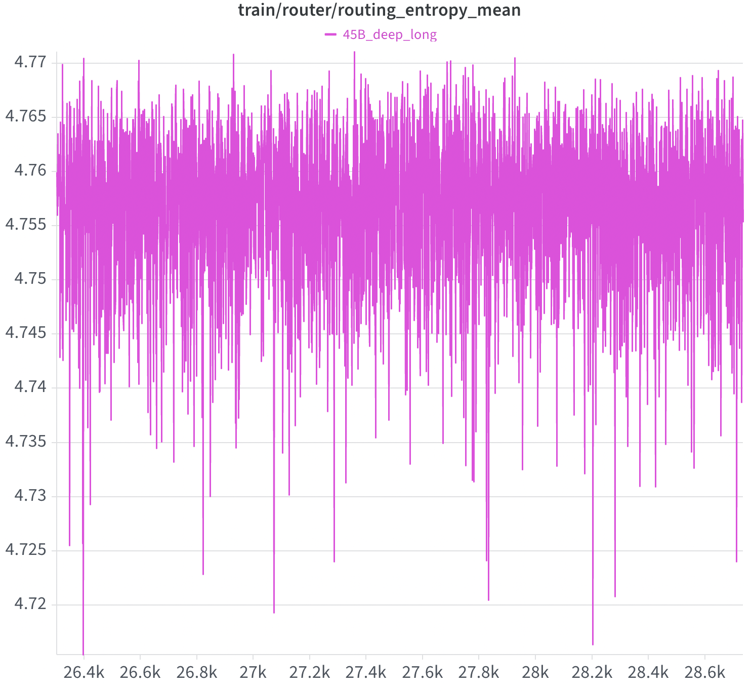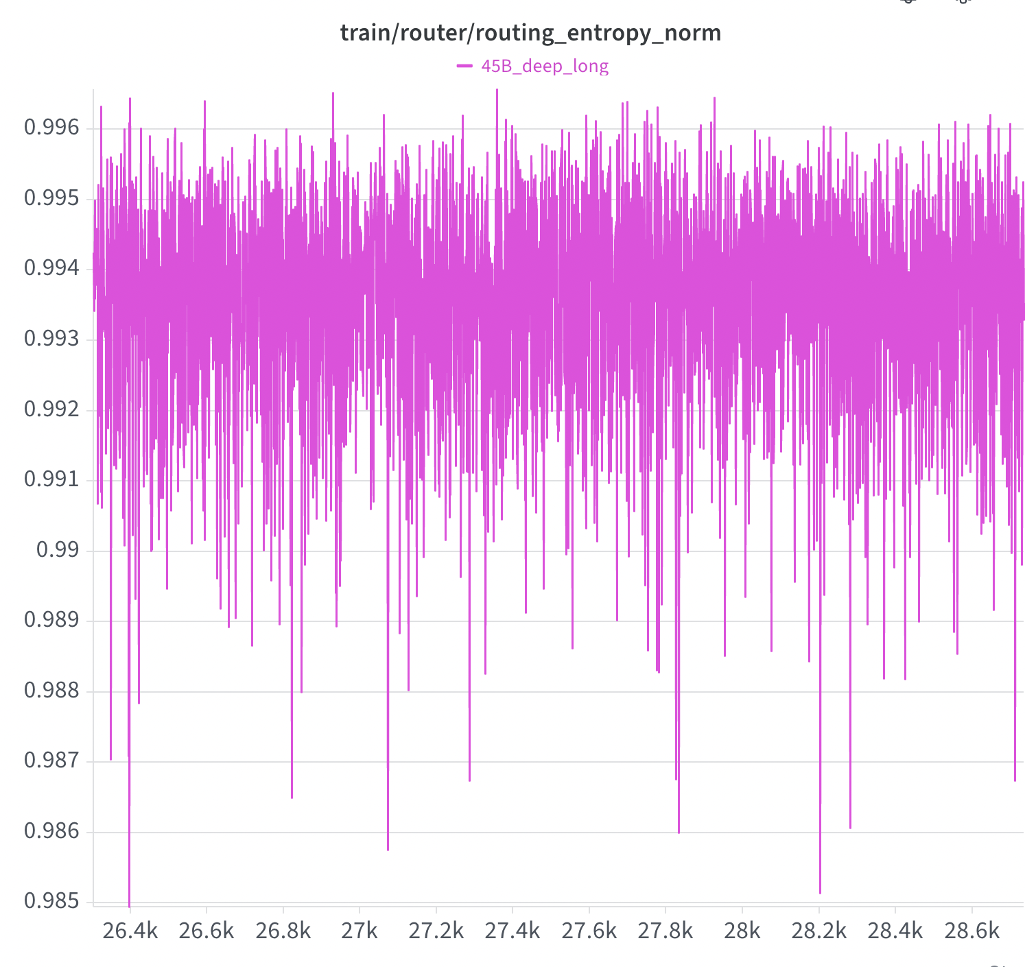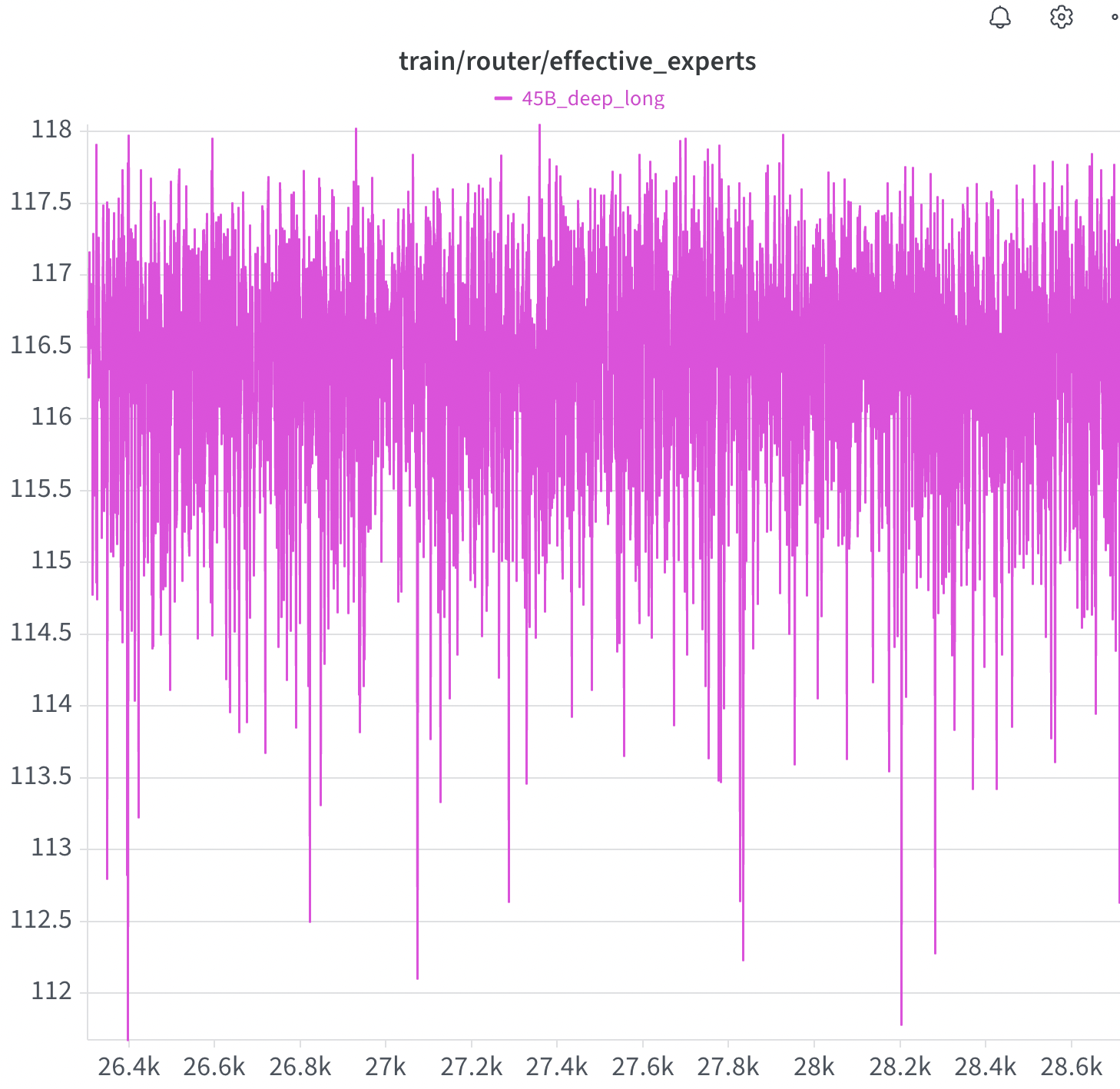For interpretability, we can also plot the routing_entropy_norm, which is $\frac{H_{r e a l}}{H_{i d e a l}}$ and a value of 1 means we're getting the perfect balance. Additionally, if we convert the routing entropy into perplexity by exponentiating it, we get the number of effective experts and as you can see, that averages around 116, so not perfect, but very good.

Figure 4: How effective experts, routing entropy norm and mean behave during training.

Note that we do not expect or get perfect balance per batch due to the fact that biases are computed for one batch and applied to the next, but on average across training, expert utilisation stays even and assignments don't get concentrated.