← Arsalan Zafar

Manifold-constrained hyper-connections

Residual connections were introduced by the ResNet paper and helped train deeper and deeper models. Attention Is All You Need brought residual connections to the transformer architecture, but Hyper-Connections expanded its capabilities by introducing multiple streams and read, write and mixing matrices. mHC improved their stability and scalability.

How it works

We start by copying our embeddings into $n$ streams, so we go from $[b,t,d_{model}]$ to $[b,t,n,d_{model}]$ where $n$ is a hyperparameter. The original DeepSeek paper used 4, but others have tried fewer streams, which still work quite well.

Our aim with mHC is to provide each sublayer (attention and FFN) the ability to read from and write into our residual stream, which is more powerful than simply adding the input to the output as done in vanilla architectures. We also want to give the model a method to mix the information across the streams, as that is a powerful bias for the model to have. It can then choose to mix information as it pleases or keep all streams separate. It can turn one of the streams into a skip connection or specialise them to the sublayers. The more control we give to the network in general, the better.

Read

With mHC, before each sublayer, the model gets to decide the input. It isn't as simple as the output of the previous layer anymore, since we now have 4 residual streams holding the information. We also need to turn the four streams into one. We do this by producing four values, which are the mixture weights of each of the streams. Then we perform a weighted combination of the four streams to get one stream. We build these weights using the input and some learned scales and biases. Eq. 1 outlines how we do this:

$$\begin{array}{}\text{(}\text{1}\text{)}& H^{pre}=\sigma ({\alpha }^{pre}(x_{input}{\varphi }^{pre})+{\beta }^{pre})\end{array}$$

Here, ${\varphi }^{pre}$ is a linear projection of the input, of shape $[n\cdot d_{model},n]$, while ${\alpha }^{pre}$ is a learned scale of shape $[1]$ and ${\beta }^{pre}$ is a learned bias per stream, of dimension $[n]$. These are both independent of input and the same for every token. We also apply the sigmoid function to get the $n$ values between 0 and 1. $H^{pre}$ is of size $[b,t,n]$, so we get 4 values per token which decide how its input should be built from its four residual vectors. $x_{input}$ is defined as $[b,t,n,d_{model}]$ and is flattened to $[b,t,n\cdot d_{model}]$ for the projection.

We then multiply $H^{pre}$ with the input to get the input to our sublayer.

$$\begin{array}{}\text{(}\text{2}\text{)}& h_{in}=H^{pre}{x}_{input}\end{array}$$

where $h_{in}$ is of shape $[b,t,d_{model}]$.

Write

After each sublayer, say attention or an FFN, we have a $[b,t,d_{model}]$ output, and we need to inject the output back into our residual stream so it can utilise it for later layers. To do this, we need to turn the single stream back into four streams, and we do this the same way as the read operation. We construct four values, which we use to scale the output of the sublayer and add to each of the inputs of our residual stream. These four values are constructed from the layer's input, not its output, using:

$$\begin{array}{}\text{(}\text{3}\text{)}& H^{post}=2\sigma ({\alpha }^{post}(x_{input}{\varphi }^{post})+{\beta }^{post})\end{array}$$

Here, ${\varphi }^{post}$ is a linear projection of the input, of shape $[n\cdot d_{model},n]$, while ${\alpha }^{post}$ is a learned scale of shape $[1]$ and ${\beta }^{post}$ is a learned bias per stream, of dimension $[n]$. These are both independent of input and the same for every token. We also apply the sigmoid function to get the $n$ values between 0 and 1, and since $\sigma (0)=0.5$, the 2× factor makes the write weights start at 1 as at the start of training we want the output to be fully written to each stream. $H^{post}$ is of size $[b,t,n]$, so we get 4 values per token which decide how much of the sublayer output should be added to each of the four residual streams. $x_{input}$ is defined as $[b,t,n,d_{model}]$.

We then multiply $H^{post}$ with the sublayer output to get what is written into each stream.

$$\begin{array}{}\text{(}\text{4}\text{)}& x_{write}=H^{post}{x}_{out}\end{array}$$

where $x_{out}$ is of shape $[b,t,d_{model}]$ and $x_{write}$ is of shape $[b,t,n,d_{model}]$. During implementation, we need to turn the $n$ values of $H^{post}$ into a column vector and $x_{out}$ into a row vector, so we can have an outer product where each of the four $n$ values multiplies the token vector to give four token vectors, one for each residual stream. In code, we do this by expanding $x_{out}$ dimension and $H^{post}$ dimensions.

# H_post.unsqueeze(-1) = [b, t, n, 1]
# x_out.unsqueeze(-2) = [b, t, 1, d_model]
out = H_post.unsqueeze(-1) @ x_out.unsqueeze(-2) # output: [b, t, n, d_model]

It might make more sense to use $x_{out}$ to compute $H^{post}$ so that output can decide how to mix itself into the residual stream, and this is likely a better alternative. However, that would make mHC sublayer-dependent and sequential, impacting efficient inference. The ability to compute all the weights from the sublayer's input, independent of its output, affords parallelism.

Mix

In between the sublayers, we'd like a way to share information between the residual streams. The DeepSeek paper found mixing alone accounts for most of the gains of mHC. We could argue that the read and write operations have some mixing built in, but the constraint of having to compress four streams into one, go through a sublayer and then fan out to four streams seems to constrain the mixing too much. A better method is to mix directly across the streams.

To mix, for each stream we need to add to it the remaining streams, but we'd like the model to have control over how much of each stream should mix with the other. This would look something like Eq. 5.

where $x_i$ is the $i$-th stream. We can see that we need 16 $w_{ij}$ values for the mixing. We can ask the model to predict these values from the input, much like $H^{post}$ and $H^{pre}$:

$$\begin{array}{}\text{(}\text{6}\text{)}& H^{res}={\alpha }^{res}(x_{input}{\varphi }^{res})+{\beta }^{res}\end{array}$$

Here, ${\varphi }^{res}$ is a linear projection of the input, of shape $[n\cdot d_{model},n^2]$, while ${\alpha }^{res}$ is a learned scale of shape $[1]$ and ${\beta }^{res}$ is a learned bias of dimension $[n^2]$. These are both independent of input and the same for every token. $H^{res}$ is of shape $[b,t,n^2]$ so we get 16 values per token, which, once normalised, are our 16 mixing ratios.

To preserve the input scale and encourage even mixing, we need to ensure that the $w_{ij}$ values used to produce each stream are non-negative and sum to one. For this, we organise our values in a $4\times 4$ matrix and ensure the rows and columns sum to one.

We can also see that the diagonal entries represent how much each stream keeps of itself, while the off-diagonal entries are how much each stream contributes to the others. By asking the rows to sum to one, we ensure that each stream takes the linear combination of the others and by asking the columns to sum to one, we ensure each stream contributes to others only that which keeps the total contributions weight sum at 1. By asking both the rows and columns to sum to one, we limit how much this matrix can stretch/amplify a unit vector. This helps stabilise training in the forward pass and backward pass. Without it, the mixing could collapse where a few streams dominate. We use the Sinkhorn–Knopp algorithm to ensure that the rows and columns sum to one by iteratively normalising them. This is done for 20 steps in the DeepSeek paper.

The Sinkhorn–Knopp algorithm is an alternating column-wise and row-wise softmax. Given an unconstrained matrix $M$ of size $n\times n$, we first make the values positive by applying exp:

$$\begin{array}{}\text{(}\text{8}\text{)}& M_{ij}^{(0)}=\exp (H_{ij}^{res})\end{array}$$

where $i$ and $j$ are the row and column indices. Next we divide each column by the sum of that column.

$$\begin{array}{}\text{(}\text{9}\text{)}& C_{ij}=\frac{M_{ij}}{\sum _k{M}_{kj}}\end{array}$$

Which causes each of the columns to sum to one. We then do the same for each of the rows, starting from $C$:

$$\begin{array}{}\text{(}\text{10}\text{)}& R_{ij}=\frac{C_{ij}}{\sum _k{C}_{ik}}\end{array}$$

Which causes the rows to sum to one. However, we can't guarantee the columns still sum to one. So we perform the column and row normalisation alternately for 20 steps and the resulting matrix will have both rows and columns summing to one. Quite simple, yet beautiful.

A naive PyTorch implementation

Here, we present a simple PyTorch implementation of mHC. A few notes to help understand the implementation:

• $\alpha$ initialisation on lines 10, 17 and 22 is a single value learnt for each read, write and mixing operation. It is the same for every token and is learnt by the model throughout training.
• $\beta$ initialisation on lines 13, 18 and 25 is $n$ values for read and write and $n^2$ values for the mixing operation. It is the same for every token and is learnt by the model throughout training.
• Since all $2n+n^2$ values for read, write and mixing depend on the same input, $x_{input}$ (x_res in the code), they can be computed once using a combined matmul as done in the gemm_projection function. If we stack the projection matrices for each of these in the width dimension, we can do one matmul and break off each of the outputs.
• For Sinkhorn, we use logsumexp to prevent underflow and overflow.
• A specific initialisation is used to encourage good mixing from the start:
  • The mixing matrix is near-identity at initialisation (after Sinkhorn), to preserve each stream's identity.
  • The write gate is fully open at initialisation, and each residual stream gets the whole sublayer output.
  • Different layers are initialised to read from different streams, to encourage more complex interactions and read patterns.

class mHC(nn.Module):
    def __init__(self, cfg, layer_idx):
        super().__init__()

        n = cfg["n"]
        d_model = cfg["d_model"]

        # Read gate: scalar scale and per-stream bias
        # [] and [n]
        self.alpha_pre = nn.Parameter(torch.tensor(0.01))
        beta_pre = torch.full((n,), -4.0)
        beta_pre[layer_idx % n] = 4.0
        self.beta_pre = nn.Parameter(beta_pre)

        # Write gate: scalar scale and per-stream bias
        # [] and [n]
        self.alpha_post = nn.Parameter(torch.tensor(0.01))
        self.beta_post = nn.Parameter(torch.zeros(n))

        # Residual mixing: scalar scale and flattened identity-biased logits
        # [] and [n*n]
        self.alpha_res = nn.Parameter(torch.tensor(0.01))
        beta_res = torch.full((n, n), -4.0)
        beta_res.fill_diagonal_(0.0)
        self.beta_res = nn.Parameter(beta_res.flatten())

        # Joint projection for input-dependent read, write and mixing gates
        # [b, t, n*d_model] @ [n*d_model, 2*n+n*n] -> [b, t, 2*n+n*n]
        self.phi = nn.Linear(n*d_model, 2*n+n*n, bias=False)

    def gemm_projection(self, x_res):
        # [b, t, n, d_model]
        b, t, n, d_model = x_res.shape

        # Flatten all residual streams
        # [b, t, n, d_model] -> [b, t, n*d_model]
        x_res_flat = x_res.reshape(b, t, n*d_model)

        # Compute inverse RMS across all streams
        # [b, t, n*d_model] -> [b, t, 1]
        r = torch.rsqrt(
            x_res_flat.pow(2).mean(-1, keepdim=True, dtype=torch.float32) + 1e-20
        )

        # Project and normalize gate logits
        # [b, t, n*d_model] @ [n*d_model, 2*n+n*n] -> [b, t, 2*n+n*n]
        output = self.phi(x_res_flat) * r

        # Split logits into read, write and residual mixing
        # [b, t, 2*n+n*n] -> [b, t, n], [b, t, n], [b, t, n*n]
        self.read_m = output[:, :, :n]
        self.write_m = output[:, :, n:2*n]
        self.mix_m = output[:, :, 2*n:]

    def read(self, x_res):
        # [b, t, n, d_model]
        b, t, n, d_model = x_res.shape

        # Generate input-dependent read weights
        # [b, t, n] * [] + [n] -> [b, t, n]
        h_pre = torch.sigmoid(self.alpha_pre * self.read_m + self.beta_pre)

        # Weighted sum of residual streams
        # [b, t, 1, n] @ [b, t, n, d_model] -> [b, t, 1, d_model]
        out = h_pre.unsqueeze(-2) @ x_res

        # [b, t, 1, d_model] -> [b, t, d_model]
        return out.squeeze(-2)

    def write(self, x_res, x_layer):
        # x_res: [b, t, n, d_model]
        # x_layer: [b, t, d_model]
        b, t, n, d_model = x_res.shape

        # Generate input-dependent write weights
        # [b, t, n] * [] + [n] -> [b, t, n]
        h_post = 2.0 * torch.sigmoid(
            self.alpha_post * self.write_m + self.beta_post
        )

        # Distribute sublayer output across residual streams
        # [b, t, n, 1] @ [b, t, 1, d_model] -> [b, t, n, d_model]
        out = h_post.unsqueeze(-1) @ x_layer.unsqueeze(-2)

        # [b, t, n, d_model]
        return out

    def mix(self, x_res):
        # [b, t, n, d_model]
        b, t, n, d_model = x_res.shape

        # Generate input-dependent residual mixing logits
        # [b, t, n*n] * [] + [n*n] -> [b, t, n, n]
        h_res = (
            self.alpha_res * self.mix_m + self.beta_res
        ).reshape(b, t, n, n)

        # Normalize into a doubly stochastic mixing matrix
        # [b, t, n, n] -> [b, t, n, n]
        h_res = self.sinkhorn(h_res)

        # Mix residual streams
        # [b, t, n, n] @ [b, t, n, d_model] -> [b, t, n, d_model]
        out_res = h_res @ x_res

        # [b, t, n, d_model]
        return out_res

    def sinkhorn(self, logits, n_iters=20):
        # logits: [b, t, n, n]
        assert logits.shape[-2] == logits.shape[-1]

        # Convert logits to FP32
        # [b, t, n, n] -> [b, t, n, n]
        z = logits.float()

        for _ in range(n_iters):
            # Normalize columns in log-space
            # [b, t, n, n] - [b, t, 1, n] -> [b, t, n, n]
            z = z - torch.logsumexp(z, dim=-2, keepdim=True)

            # Normalize rows in log-space
            # [b, t, n, n] - [b, t, n, 1] -> [b, t, n, n]
            z = z - torch.logsumexp(z, dim=-1, keepdim=True)

        # Convert log probabilities to mixing weights
        # [b, t, n, n] -> [b, t, n, n]
        return z.exp().to(logits.dtype)

Results

The plot below shows the held-out cross-entropy loss of a vanilla 124M model vs the same model with mHC trained for 2.5B tokens on the FineWeb-Edu dataset. We can see a ~1% improvement in validation loss. That might not look like much, but the difference is still growing. mHC also has synergies with Engram.

For a deeper analysis of mHC, please review the Nenya technical report.

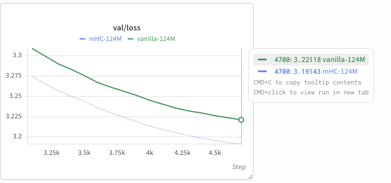
Figure 1: Held-out validation loss comparing vanilla transformer vs vanilla transformer with mHC.